Here we present a yield curve interpolation method, one that’s based on conditioning a stochastic model on a set of market yields. The concept is closely related to a Brownian bridge where you generate scenario according to an SDE, but with the extra condition that the start and end of the scenario’s must have certain values. In this paper we use Gaussian process regression to generalization the Brownian bridge and allows for more complicated conditions. As an example, we condition the Vasicek spot interest rate model on a set of yield constraints and provide an analytical solution.
The resulting model can be applied in several areas:
- Monte Carlo scenario generation
- Yield curve interpolation
- Estimating optimal hedges, and the associated risk for non tradable products
Overall, this technique provides an analytical solution for the conditional scenario probability density function (pdf). Scenario generation can be accomplished by sampling from that distribution. A different application is to calculate the average yield as a function of maturity (the average of the scenario’s), which can be viewed as a interpolation method. Yet another applications is to use the relationships between yield to estimate hedges based on the relationship between interpolated yields and the available yields from quoted products.
The Vasicek Model for Interest Rates
The Vasicek model is one of the earliest mathematical models for interest rates, introduced by Oldřich Vašíček in 1977. Vašíček, a Czech-American financial economist, developed this model to describe how daily interest rates evolve over time in a stochastic (random) manner while still tending toward a long-term average level. The key feature of the model is mean reversion, meaning that if interest rates are too high, they tend to fall back, and if they are too low, they tend to rise.
The stochastic differential equation (SDE) for the Vasicek model is:
![\[d r_t = \kappa \left( \Theta - r_t \right) dt + \sigma dW_t\]](https://www.sitmo.com/wp-content/ql-cache/quicklatex.com-35dbbb99c1e0911dcd2623678228b08e_l3.png "Rendered by QuickLaTeX.com")
In this equation:
 is the interest rate at time
  .
. (often called the “speed of mean reversion”) controls how quickly moves toward the long-term average
  .
.- is the long-term mean interest rate, the level to which rates tend to revert over time.
 is the volatility, which determines how much randomness affects the interest rate movements.
 represents a random shock (a Wiener process), modeling unpredictable fluctuations in interest rates.
The first term,  ensures mean reversion: if is above , it decreases, and if it is below, it increases. The second term,
  , introduces randomness, making sure that interest rates don’t follow a perfectly predictable path.
Generating Random Paths of Daily Interest Rates
To understand how interest rates evolve over time under the Vasicek model, we need to generate random paths for . It might be tempting to directly translate the stochastic differential equation (SDE) into a discrete simulation equation, such as:
![\[r_{t+\Delta t} = r_t + \kappa (\Theta - r_t) \Delta t + \sigma \sqrt{\Delta t} \, Z_t\]](https://www.sitmo.com/wp-content/ql-cache/quicklatex.com-b354141ea1e44126374262ad672de938_l3.png "Rendered by QuickLaTeX.com")
where  is a standard normal random variable. However, this is not an exact solution and introduces discretization error. Fortunately, there is an exact simulation formula, meaning we can generate values of without approximation errors.
The exact solution for at time is:
![\[r_t = r_0 e^{-\kappa t} + \Theta \left( 1 - e^{-\kappa t} \right) + \sigma \sqrt{\frac{1 - e^{-2\kappa t}}{2\kappa}} Z_t\]](https://www.sitmo.com/wp-content/ql-cache/quicklatex.com-416649577440d7a074d879d2887bc6d4_l3.png "Rendered by QuickLaTeX.com")
where . The plot below (Fig 1) shows 5 random interest rate paths.
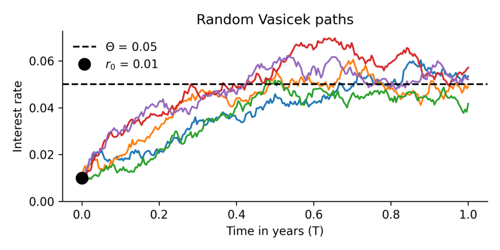
 and move towards the long-term mean of
  .
.The following Python function demonstrates how to generate a random Vasicek path using the exact simulation formula:
import numpy as np

def vasicek_random_path(r0, theta, kappa, sigma, T, dt):
    """
    Simulate a random path for the Vasicek interest rate model using the exact solution.

    Parameters:
    r0     : float  - Initial interest rate
    theta  : float  - Long-term mean interest rate
    kappa  : float  - Speed of mean reversion
    sigma  : float  - Volatility
    T      : float  - Total simulation time
    dt     : float  - Time step

    Returns:
    times  : ndarray - Array of time points
    rates  : ndarray - Simulated interest rate path
    """
    times = np.arange(0, T + dt, dt)
    rates = np.zeros_like(times)
    rates[0] = r0

    for i in range(1, len(times)):
        t = times[i]
        Z = np.random.randn()  # Standard normal variable
        rates[i] = (
            r0 * np.exp(-kappa * t) +
            theta * (1 - np.exp(-kappa * t)) +
            sigma * np.sqrt((1 - np.exp(-2 * kappa * t)) / (2 * kappa)) * Z
        )

    return times, rates
Mean, Variance, and Covariance of the Vasicek Model
Once we have a stochastic process, we often want to describe its expected behavior and uncertainty over time. The Vasicek model allows us to compute the expected value (mean), variance, and covariance of the interest rate at time .
The expected value of given an initial value  is:
is:
![\[E[r_t \mid r_0] = e^{-\kappa t} \left[ r_0 + \Theta \left( e^{\kappa t} - 1 \right) \right]\]](https://www.sitmo.com/wp-content/ql-cache/quicklatex.com-2d91ad5e0664b7a756626cb25f0e0b8c_l3.png "Rendered by QuickLaTeX.com")
This formula shows that as time increases, moves toward the long-term mean . The rate of this movement is controlled by .
The variance of measures its uncertainty:
![\[\text{Var}[r_t] = \sigma^2 \left( \frac{1 - e^{-2\kappa t}}{2\kappa} \right)\]](https://www.sitmo.com/wp-content/ql-cache/quicklatex.com-a69b454065f5f5dcd3d51f04e4dfb664_l3.png "Rendered by QuickLaTeX.com")
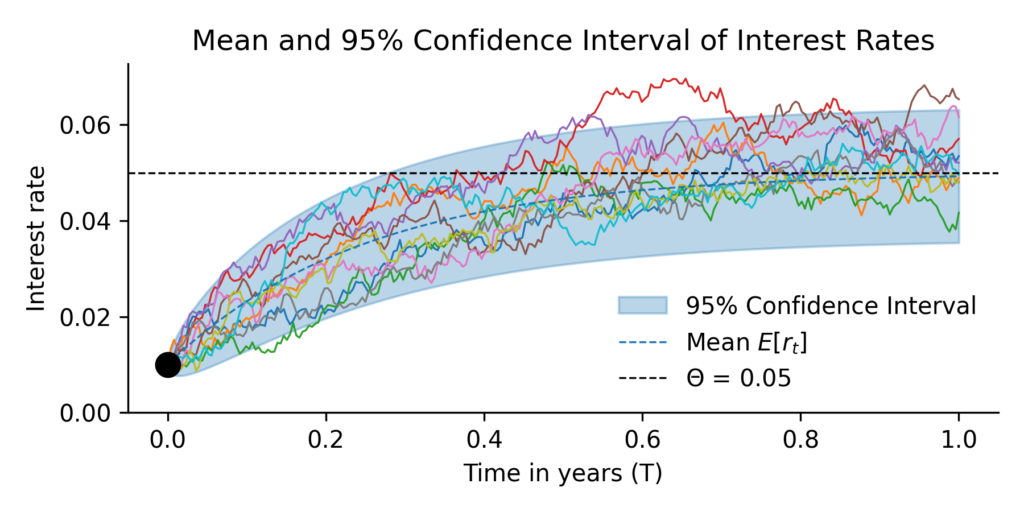
The longer we simulate, the higher the variance, until it stabilizes at a long-term level.
The covariance between two points in time, and  , is:
, is:
![\[\text{Cov}[r_t, r_u] = \frac{\sigma^2}{2\kappa} e^{-\kappa(t+u)} \left( e^{2\kappa \min(t,u)} - 1 \right)\]](https://www.sitmo.com/wp-content/ql-cache/quicklatex.com-5794dba651fbcf5a782acc8b5c1a3e3e_l3.png "Rendered by QuickLaTeX.com")
This tells us how correlated different times are in the Vasicek model. The closer two time points are, the stronger their correlation.
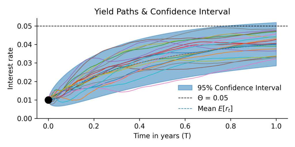
The next plot uses the mean and variane equations to lpot the mean and the 95% confidence interval of the random price path.
Below are the Python functions for these mean, variance and covariance equations:
import numpy as np
import matplotlib.pyplot as plt

def vasicek_mean(r0, theta, kappa, t):
    """Compute the expected value E[r_t | r_0] for the Vasicek model."""
    return np.exp(-kappa * t) * (r0 + theta * (np.exp(kappa * t) - 1))

def vasicek_var(sigma, kappa, t):
    """Compute the variance Var[r_t] for the Vasicek model."""
    return (sigma ** 2) * (1 - np.exp(-2 * kappa * t)) / (2 * kappa)

def vasicek_cov(sigma, kappa, t, u):
    """Compute the covariance Cov[r_t, r_u] for the Vasicek model."""
    return (sigma ** 2 / (2 * kappa)) * np.exp(-kappa * (t + u)) * (np.exp(2 * kappa * min(t, u)) - 1)
Yield and Interest Rates
In fixed income markets, money is borrowed and lent over fixed periods, from one month to thirty years or more. The interest rate associated with a specific maturity reflects the cost of borrowing or the return on lending over that period. When we talk about the yield, we refer to the interest rate as a function of time to maturity.
Importantly, the yield is not the rate at a single moment, it’s the average rate you earn (or pay) over the full lifetime of the loan.
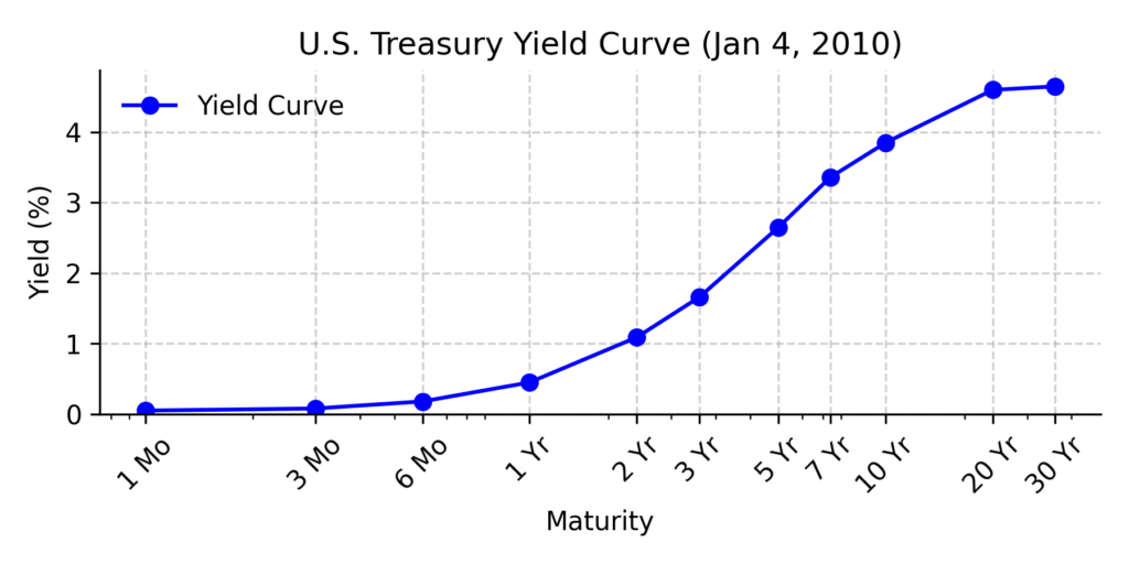
The U.S. Department of the Treasury publishes historicalk daily yield curve data. These reflect the yields for different maturities based on government bond prices. You can explore this data at: U.S. Treasury Yield Curve Data
The plot below shows the U.S. Treasury yield curve on January 4, 2010. The x-axis represents time to maturity, and the y-axis shows the corresponding annual yield (in percent).
The spot interest rate of the Vasicek model is a Gaussian process, and the yield can be shown to be Gaussian process as well. The yield at time is defined as the average compounded rate over the time interval ![[0,t]](https://www.sitmo.com/wp-content/ql-cache/quicklatex.com-90e01491191ec1f4f923174ff69a7a73_l3.png "Rendered by QuickLaTeX.com") :
:
![\[Y_t = \frac{1}{t} \int_0^t r_u \, du\]](https://www.sitmo.com/wp-content/ql-cache/quicklatex.com-b620e9564ea7b4197fa175b61cbe954a_l3.png "Rendered by QuickLaTeX.com")
This means that instead of looking at the instantaneous short rate , we take the time-averaged rate up to .
To obtain properties of  , we integrate the Vasicek model. The process requires computing expectations, variances, and covariances of the integral of . While the full derivation involves stochastic calculus, we skip the details and directly present the solution:
![\[E[Y_t] =\Theta + \frac{(r_0 - \Theta)}{-\kappa t} \left(e^{-\kappa t} - 1\right)\]](https://www.sitmo.com/wp-content/ql-cache/quicklatex.com-24d411bca12691aebc728457d55d05f2_l3.png "Rendered by QuickLaTeX.com")
![\[\text{Var}[Y_t] =\frac{\sigma^2}{2 \kappa^3 t^2} \left(2 \kappa t - 3 + 4 e^{-\kappa t} - e^{-2\kappa t} \right)\]](https://www.sitmo.com/wp-content/ql-cache/quicklatex.com-1214524c7c9661bde0a0fad8f82c02a5_l3.png "Rendered by QuickLaTeX.com")
![\[\text{Cov}[Y_t, Y_u] =\frac{\sigma^2}{2 \kappa^3 t u} \left(2 \kappa t - 2 + 2 e^{-\kappa t} + 2 e^{-\kappa u} - e^{\kappa (t - u)} - e^{-\kappa (t + u)} \right)\]](https://www.sitmo.com/wp-content/ql-cache/quicklatex.com-d8c8c6a396498a44eff335cbfbc1b008_l3.png "Rendered by QuickLaTeX.com")
Just like the spot rate, these equations describe how the yield behaves over time and how yields at different time points are related. The covariance equation shows that yields are highly correlated over time due to the fact that yields to different maturity have shared overlapping initial periods.
Below is the same plot as before, but this time for yield instead of rates. These yields are ‘realised yields’, the running average of spot rate paths.
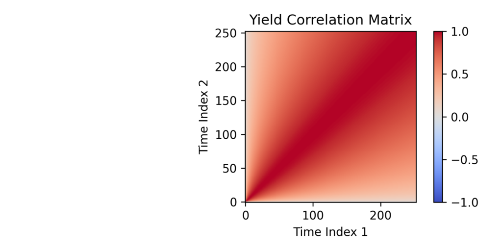
And here is a plot of the correlations between different maturities. Yields at nearby maturities tend to move together, which shows up as strong correlations along the diagonal. As maturities get further apart, the correlation weakens. Longer maturities tend to remain more correlated with each other than shorter ones. This happens because long-term yields average over a longer shared initial period, which creates more stable, closely linked behavior.
Below are Python functions for these yield equations:
def vasicek_yield_mean(r0, theta, kappa, t):
    """Compute the expected value E[Y_t] of the yield under the Vasicek model."""
    return theta + (r0 - theta) / (-kappa * t) * (np.exp(-kappa * t) - 1)

def vasicek_yield_var(sigma, kappa, t):
    """Compute the variance Var[Y_t] of the yield under the Vasicek model."""
    return sigma ** 2 / (2 * kappa ** 3 * t ** 2) * (2 * kappa * t - 3 + 4 * np.exp(-kappa * t) - np.exp(-2 * kappa * t))

def vasicek_yield_cov(sigma, kappa, t1, t2):
    """Compute the covariance Cov[Y_t, Y_u] of the yield under the Vasicek model."""
    t = min(t1, t2)
    u = max(t1, t2)
    return sigma ** 2 / (2 * kappa ** 3 * t * u) * (
        2 * kappa * t - 2 + 2 * np.exp(-kappa * t)
        + 2 * np.exp(-kappa * u) - np.exp(kappa * (t - u)) - np.exp(-kappa * (t + u))
    )
Gaussian Processes
The Vasicek model is a Gaussian Process, meaning that at any set of time points  , the corresponding interest rates (or yields) follow a multivariate normal distribution:
![\[\mathbf{r} \sim \mathcal{N}(\boldsymbol{\mu}, \boldsymbol{\Sigma})\]](https://www.sitmo.com/wp-content/ql-cache/quicklatex.com-c4ae9078e445b03ef68efc3429419610_l3.png "Rendered by QuickLaTeX.com")
where:
 is the vector of expected values
 ![E[r_t]](https://www.sitmo.com/wp-content/ql-cache/quicklatex.com-66715019251a56cebb1f47fa20c2f66a_l3.png "Rendered by QuickLaTeX.com") .
. is the covariance matrix
 ![\text{Cov}[r_t, r_u]](https://www.sitmo.com/wp-content/ql-cache/quicklatex.com-eb603bbad5c1dd8f6a42dbc789e6f6ce_l3.png "Rendered by QuickLaTeX.com") .
.
This structure allows us to generate Vasicek paths in two ways:
- Step-by-step simulation, as we did earlier.
- Directly sampling paths from the multivariate Gaussian, which is computationally efficient and fully consistent with the model’s statistical structure.
A Gaussian Process is more than just a multivariate normal distribution, it is a continuous stochastic process. Instead of being defined only at discrete time points, it is fully described by two functions:
- The mean function
![m(t) = E[r_t]](https://www.sitmo.com/wp-content/ql-cache/quicklatex.com-9446088e92a939fffcb302f4e6f4be11_l3.png "Rendered by QuickLaTeX.com") , which gives the expected value at any time.
, which gives the expected value at any time. - The covariance function
![k(t, u) = \text{Cov}[r_t, r_u]](https://www.sitmo.com/wp-content/ql-cache/quicklatex.com-386342c6d5f2e9de9b3c4c5d3a556f4b_l3.png "Rendered by QuickLaTeX.com") , which determines how correlated different time points are.
, which determines how correlated different time points are.
This means we can model the Vasicek process at any level of detail, zooming in as much as we like without being restricted to predefined time steps.
However, in practice, we always work with finite-dimensional representations. Whether in simulations, data analysis, or financial modeling, we evaluate the process at specific time points, forming vectors and matrices instead of an infinite-dimensional function. The continuous GP perspective mainly gives us the flexibility to choose any resolution.
For example, if we observe interest rates daily, we are effectively seeing a finite sample from the underlying continuous function. When simulating paths, we do not generate an infinitely detailed function but rather a discrete approximation at selected time steps.
To illustrate this, we now generate sample paths from the Gaussian Process representation of the Vasicek model. Instead of constructing paths step by step, we sample them directly from the multivariate Gaussian defined by the Vasicek mean and covariance functions.
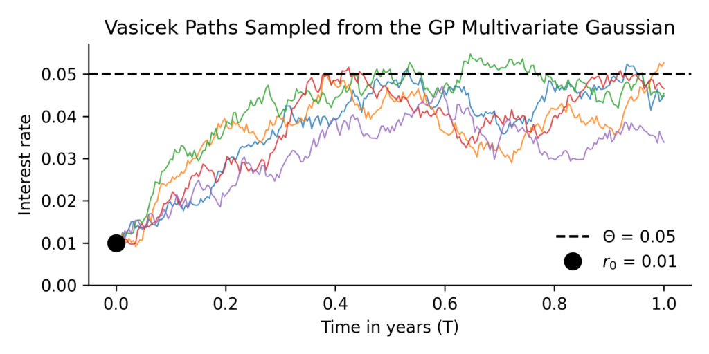
Below is the main element of the used to generate this plot. We first contruct a mean vector and covariance matrix at the resolution we are interested in, and then draw radom samples -the paths- from the multivariate Guassian.
# Function to compute the mean vector
def vasicek_mean_vector(r0, theta, kappa, time_grid):
    return np.array([np.exp(-kappa * t) * (r0 + theta * (np.exp(kappa * t) - 1)) for t in time_grid])

# Function to compute the covariance matrix
def vasicek_cov_matrix(sigma, kappa, time_grid):
    d = len(time_grid)
    cov_matrix = np.zeros((d, d))
    for i in range(d):
        for j in range(d):
            t, u = time_grid[i], time_grid[j]
            cov_matrix[i, j] = (sigma ** 2 / (2 * kappa)) * np.exp(-kappa * (t + u)) * (np.exp(2 * kappa * min(t, u)) - 1)
    return cov_matrix

# Compute mean and covariance matrix
mu = vasicek_mean_vector(r0, theta, kappa, time_grid)
sigma_matrix = vasicek_cov_matrix(sigma, kappa, time_grid)

# Sample paths from the multivariate Gaussian
num_samples = 5
sampled_paths = np.random.multivariate_normal(mu, sigma_matrix, size=num_samples)
From Gaussian Processes to Conditional Distributions
So far, we have established that the Vasicek model is a Gaussian Process, meaning that interest rates or yields at different time points follow a multivariate normal distribution. This gives us a powerful tool: we can describe the full statistical structure of the process using its mean and covariance functions.
Now, we take this one step further. Instead of considering the entire yield curve as a free-floating random process, we often have some known values -for example, market quotes for certain maturities. However, the yields at other maturities remain unknown and need to be interpolated in a way that is fully consistent with the Vasicek dynamics.
This is where conditional distributions come in. By conditioning the yield curve on known market quotes, we can compute the most likely values for the missing points while preserving the statistical relationships dictated by the Vasicek model.
Lets now first look at the equations of a conditional distributions. The multivariate Gaussian distribution is given by:
![\[\mathcal{N}(\mathbf{Y} \mid \boldsymbol{\mu}, \boldsymbol{\Sigma}) =\frac{\exp \left( -\frac{1}{2} (\mathbf{Y} - \boldsymbol{\mu})^T \boldsymbol{\Sigma}^{-1} (\mathbf{Y} - \boldsymbol{\mu}) \right)}{\sqrt{(2\pi)^d |\boldsymbol{\Sigma}|}}\]](https://www.sitmo.com/wp-content/ql-cache/quicklatex.com-4b6cb448c0561537d28bc872a6fe0190_l3.png "Rendered by QuickLaTeX.com")
where:
- is the mean vector.
- is the covariance matrix.
 is the determinant of .
To define conditional distributions, we partition our variables into:
- A set of known (observed) values
 .
. - A set of unknown (free) values
 .
.
Writing this in block matrix form:
![\[\mathbf{Y} =\begin{bmatrix}\mathbf{z} \\\mathbf{f}\end{bmatrix}\sim\mathcal{N}\left(\begin{bmatrix}\boldsymbol{\mu_z} \\\boldsymbol{\mu_f}\end{bmatrix},\begin{bmatrix}\boldsymbol{\Sigma_{zz}} & \boldsymbol{\Sigma_{zf}} \\\boldsymbol{\Sigma_{fz}} & \boldsymbol{\Sigma_{ff}}\end{bmatrix}\right)\]](https://www.sitmo.com/wp-content/ql-cache/quicklatex.com-c4945a067ed34f01bffe153d9cb626c0_l3.png "Rendered by QuickLaTeX.com")
The conditional distribution of given follows a Gaussian distribution:
![\[\mathbf{f} \mid \mathbf{z} \sim\mathcal{N} (c_1 \mathbf{z} + c_2, c_3)\]](https://www.sitmo.com/wp-content/ql-cache/quicklatex.com-ae2aefea0b4789e80a91b975cbf9e7fd_l3.png "Rendered by QuickLaTeX.com")
where:


Visualizing Conditional Gaussian Processes
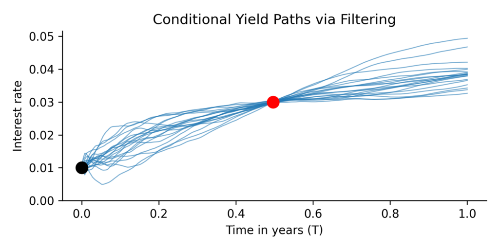
To build intuition, we can visualize how the equations above apply to yield curves. The idea of conditioning is closely tied to the notion of filtering: we simulate many possible yield curves and only keep the ones that match known information. In our case, this known information is a specific market yield (marked as a red dot).
The figure below demonstrates this idea. We simulate a large number of random Vasicek paths using the SDE and then discard all paths that do not pass close to the red dot. What remains are paths that are consistent with both the stochastic Vasicek model, but only those where a specific condition is met. This is the essence of conditioning.
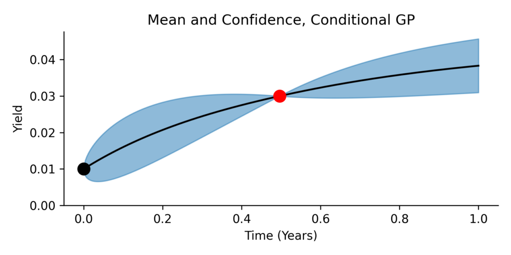
While filtering is intuitive, it is inefficient. The purpose of the conditional equations from the previous section it to allow us to compute the conditional distribution analytically. The next plot shows the mean and 95% confidence band of the conditional Gaussian process. This result is mathematically equivalent to the filtering-based approach, but computed directly using the formulas for conditional mean and covariance.
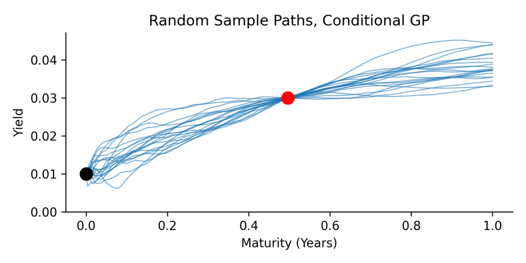
We can also draw random paths from this conditional Gaussian. These paths follow the Vasicek dynamics and are consistent with the observed yield value. These samples resemble the filtered paths from earlier.
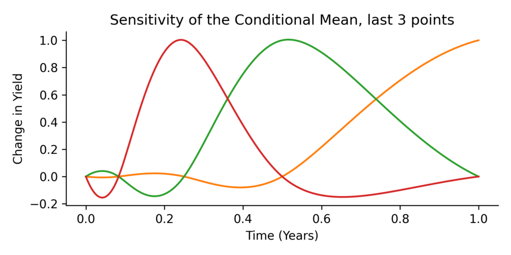
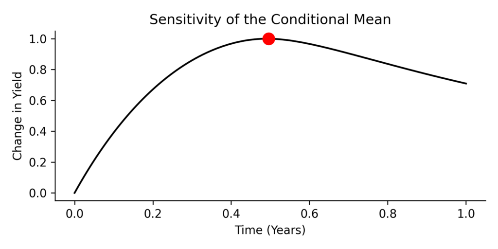
Lastly, we visualize the sensitivity of the conditional mean to the conditioning variable. The curve below shows how a small upward shift in the red dot (the observed yield) would propagate across the rest of the yield curve. This corresponds to the matrix (  ) in the conditional equations. Each point on the black curve shows how sensitive that time point is to the observed yield value. The sensitivity can be really helpfull when we want to determine proxy hedges.
The Python code used for this plot, based on for the equations above:
import numpy as np

import scipy.stats as stats

def compute_conditional_params(mean, cov, mask):
    """
    Compute c1, c2, c3 for a Gaussian conditional distribution.

    Parameters:
    mean : ndarray - Mean vector of the full distribution.
    cov  : ndarray - Covariance matrix of the full distribution.
    mask : ndarray - Boolean mask where True indicates observed variables.

    Returns:
    c1, c2, c3 : Conditional distribution parameters.
    """
    mask = np.asarray(mask, dtype=bool)
    not_mask = ~mask

    # Partition mean vector and covariance matrix
    mu_z, mu_f = mean[mask], mean[not_mask]
    Sigma_zz = cov[np.ix_(mask, mask)]
    Sigma_fz = cov[np.ix_(not_mask, mask)]
    Sigma_ff = cov[np.ix_(not_mask, not_mask)]

    # Compute conditional parameters
    Sigma_zz_inv = np.linalg.inv(Sigma_zz)
    c1 = Sigma_fz @ Sigma_zz_inv
    c2 = mu_f - c1 @ mu_z
    c3 = Sigma_ff - c1 @ Sigma_fz.T

    return c1, c2, c3

def compute_conditional_distribution(mean, cov, mask, observed_values):
    """
    Compute the conditional mean and covariance given observations.

    Parameters:
    mean            : ndarray - Mean vector of the full distribution.
    cov             : ndarray - Covariance matrix of the full distribution.
    mask            : ndarray - Boolean mask indicating observed variables.
    observed_values : ndarray - Values of the observed variables.

    Returns:
    conditional_mean : ndarray - Mean vector of the conditional distribution.
    conditional_cov  : ndarray - Covariance matrix of the conditional distribution.
    """
    c1, c2, c3 = compute_conditional_params(mean, cov, mask)
    conditional_mean = c1 @ observed_values + c2
    conditional_cov = c3

    return conditional_mean, conditional_cov
Market-Adjusted Conditioning
So far, we’ve conditioned the Gaussian process on exact yield values. While this is mathematically valid, it’s not entirely realistic. In the real world, we don’t truly know what the yield will be in the future, even if we have a current market quote. The observed yields represent present expectations, not future certainties.
The Gaussian Process view offers us a simple and principled way to deal with this: instead of treating market yields as known constants, we can treat them as random variables with a given distribution. This allows us to soften the conditioning and build a more realistic model of yield uncertainty.
We call this approach market-adjusted conditioning.
Let’s revisit what happens in standard conditioning. We partition the yield vector into:
- A set of observed variables , in the example below we will use 4 quoted market yields.
- A set of free variables , representing yields at other maturities we want to interpolate.
We’ve seen that if we condition on exact values for , the posterior distribution of becomes:
![\[\mathbf{f} \mid \mathbf{z} \sim \mathcal{N}(c_1 \mathbf{z} + c_2, \; c_3)\]](https://www.sitmo.com/wp-content/ql-cache/quicklatex.com-611e5551215ccdb22db8bec03f9d2241_l3.png "Rendered by QuickLaTeX.com")
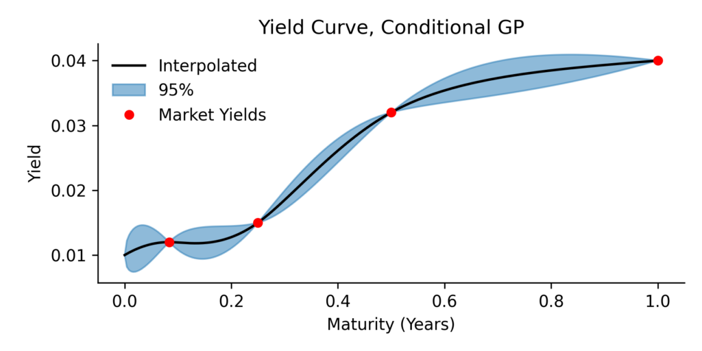
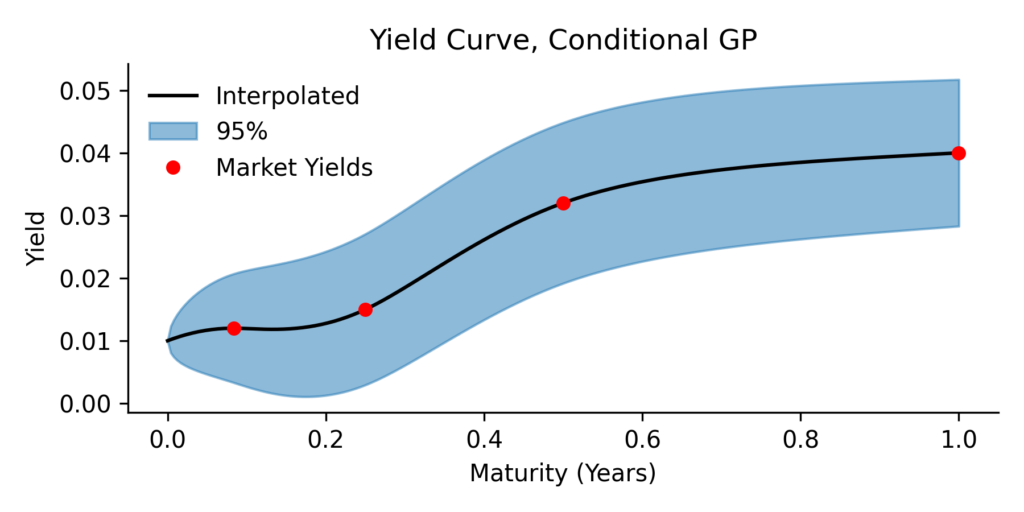
The next plot show a possible solution, where we have conditioned the yield curve on 4 market yields.
But instead of conditioning on a fixed , we now assume that itself is distributed as:
![\[\mathbf{z} \sim \mathcal{N}(\boldsymbol{\mu_z}, \boldsymbol{\Sigma_{zz}})\]](https://www.sitmo.com/wp-content/ql-cache/quicklatex.com-8b394559f526364861b4461862b0517d_l3.png "Rendered by QuickLaTeX.com")
Here,  is simply the market yield quotes (red dots), and
  is estimated using the Vasicek model (the correlations and variances between the red dots).
From this setup, we derive the posterior distribution of the remaining yields by combining the conditional and the new marginal:
![\[\mathbf{f} \sim \mathcal{N}(c_1 \boldsymbol{\mu_z} + c_2, \; c_3 + c_1 \boldsymbol{\Sigma_{zz}} c_1^\top)\]](https://www.sitmo.com/wp-content/ql-cache/quicklatex.com-2d5e23762fd1bc57ef3de228edfb50bc_l3.png "Rendered by QuickLaTeX.com")
This equation is almost identical to the classical conditioning formula, but now the mean is nudged by our belief , and the covariance accounts for the uncertainty in .
This posterior distribution is a useful outcome of applying Gaussian Processes to yield curve modeling. Here’s a brief recap:
We started with the Vasicek model, from which we derived expressions for the expected yield as a function of maturity, as well as the covariance between yields at different maturities. These two components -a mean function and a covariance function- are the foundation of Gaussian Process Regression.
By using properties of the multivariate Gaussian distribution, we obtained analytical formulas for the conditional mean and conditional covariance. This allows us to model yield curves that are consistent with observed market data.
Finally, we extended the framework by treating the observed yields themselves as uncertain, not fixed values, but random variables with their own distributions. This gives us a flexible way to combine market information with a probabilistic model of future yield behavior.
As a bonus, we have the sensitivity plot of the mean towards changes the last 3 market conditions. When we interpolate the mean yield based on multiple market values we will have multiple sensitivity curves.