Using Fractional Brownian Motion in Finance: Simulation, Calibration, Prediction and Real World Examples

Long Memory in Financial Time Series

In finance, it is common to model asset prices and volatility using stochastic processes that assume independent increments, such as geometric Brownian motion. However, empirical observations suggest that many financial time series exhibit long memory or persistence. For example, volatility shocks can persist over extended periods, and high-frequency order flow often displays non-negligible autocorrelation. To capture such behavior, fractional Brownian motion (fBm) introduces a flexible framework where the memory of the process is governed by a single parameter: the Hurst exponent.

From Brownian to Fractional: The Role of the Hurst Exponent

The Hurst exponent was originally introduced to describe long-term dependence in hydrology. In the 1950s, Harold Edwin Hurst was tasked with managing the design of reservoirs for the Nile River. A critical challenge was to ensure that the reservoir system could absorb long-term fluctuations in annual flood levels, which had a direct impact on agriculture and water availability. During this work, Hurst observed that annual water levels displayed persistent deviations from the mean over long periods. This behavior couldn’t be explained by classical models with independent random variables. Instead, he found that the standard deviation of aggregated water levels increased faster than , suggesting long-memory dynamics.

This idea led to range-scale analysis, which examines how the variability of a signal grows with the length of the observation window. For standard Brownian motion or i.i.d. noise, we know that the standard deviation scales as:

   

If the process has memory, this scaling generalizes to:

   

where is the duration of the window (or time scale), and is the Hurst exponent, which determines the scaling behavior.

with capturing the presence of persistence or anti-persistence .

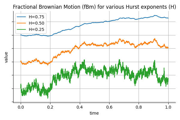
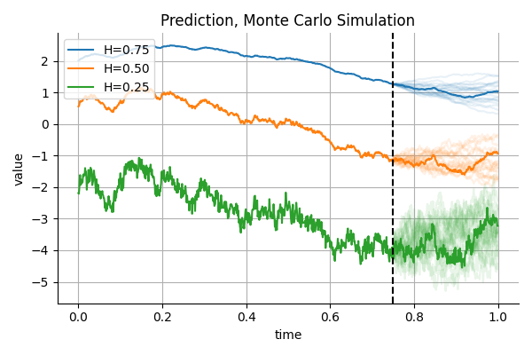
To build intuition, the figure below shows three sample paths of fractional Brownian motion, each with a different Hurst exponent . The only difference between them is how past and future values are correlated. The blue curve with is smooth and persistent, it tends to keep moving in the same direction. The orange path with behaves like standard Brownian motion, with no memory: its increments are independent. The green path with
is anti-persistent, it frequently reverses direction. The Hurst exponent controls the “roughness” of the path and its tendency to trend or revert.

The reason (H) can deviate from (0.5) is because we can allow correlation across observations. To understand this, consider a sum sequence of two independent standard normal variables, . Then , and the standard deviation grows like . However, if and are correlated, the variance of their sum becomes:

   

So, e.g. when , the standard deviation becomes 2, which corresponds to a Huste exponent of . The same logic extends to long sequences: memory in the form of persistent positive or negative correlation changes the rate at which variance accumulates over time. This is precisely what the Hurst exponent measures.

Range-Scale Analysis and the Geometry of fBm

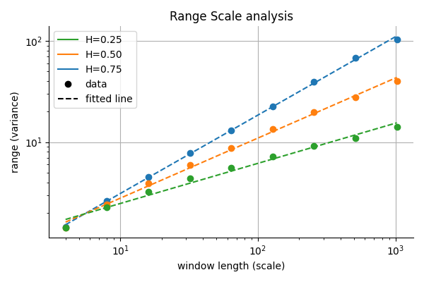
A key empirical technique for estimating is range-scale analysis. This method relies on the fact that the rescaled range of a process grows as a power-law in the window size:

   

Taking logarithms,

   

Hence, plotting against gives a straight line with slope .

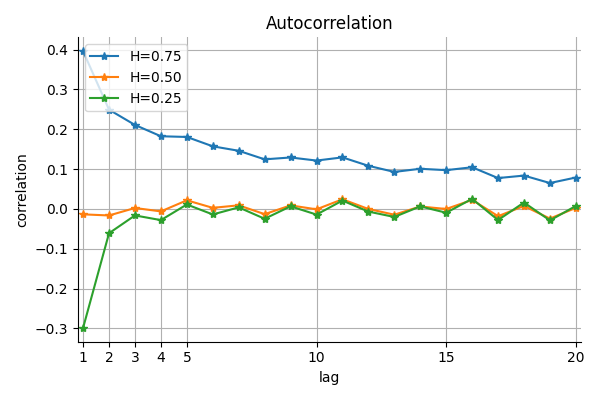
Covariance and Autocorrelation Structure

The covariance function of fractional Brownian motion is given by:

   

This structure encodes long-range dependence and determines how values at different times relate to each other. For example, when sampling fBm at times (t = 1, 2, 3, 4) with (H = 0.75), the covariance matrix becomes:

   

You can use the two function below for computing the autocorrelation and covariance matrix for fBm:

def fgn_autocovariance(n, H, dt=None):
    """
    Autocovariance function for fractional Gaussian noise (fGn).

    γ(k) = 0.5 * (|k+1|^{2H} - 2|k|^{2H} + |k-1|^{2H}) * dt^{2H}
    """
    if dt is None:
        dt = 1.0 / n
    k = np.arange(n)
    gamma = 0.5 * (np.abs(k + 1)**(2 * H) - 2 * np.abs(k)**(2 * H) + np.abs(k - 1)**(2 * H))
    return gamma * dt**(2 * H)

def fgn_covariance_matrix(n, H, dt=None):
    """
    Covariance matrix for fractional Gaussian noise (fGn).
    """
    autocov = fgn_autocovariance(n, H, dt=dt)
    cov_matrix = np.fromfunction(lambda i, j: autocov[np.abs(i - j)], (n, n), dtype=int)
    return cov_matrix

Simulating fBm

Once we understand the covariance structure of fractional Brownian motion, we can simulate its sample paths. This is important not only for theoretical analysis but also for practical tasks such as stress testing, synthetic data generation, or Monte Carlo simulation.

There are several known methods for simulating fBm. Some of the fastest include the Cholesky decomposition of the full covariance matrix, circulant embedding using the Fast Fourier Transform (FFT), and Davies–Harte methods, which exploit spectral properties. However, these methods either scale poorly with memory (e.g., for Cholesky) or can fail if the covariance matrix is not sufficiently positive definite, especially when simulating irregular time intervals or very small values of .

A more robust alternative is Hosking’s method, proposed by J.R.M. Hosking in 1984. This approach does not construct the entire covariance matrix explicitly. Instead, it generates the path incrementally, one step at a time, using the autocovariance function of fractional Gaussian noise (fGn) and recursive conditioning. It guarantees a valid Gaussian process regardless of the Hurst exponent or sample size.

The core idea is to generate fractional Gaussian noise (the increments of fBm) by recursively applying conditional expectations and variances, much like how a Kalman filter operates. At each step, the new value is computed as a linear combination of past values, weighted according to the known autocovariance structure. This is why it makes sense to present this method right after discussing the autocovariance and correlation functions—they are the mathematical backbone of the recursion.

While Hosking’s method is not the fastest (it runs in time due to the nested loops), it is numerically stable and accurate, making it a reliable choice for simulations where precision is more important than speed.

Below is a full implementation of fBm generation using this method:

def generate_fgn_hosking(n, H, dt=None):
    """
    Generate fractional Gaussian noise (fGn) using the Hosking method.
    """
    gamma = fgn_autocovariance(n, H, dt)
    fgn = np.zeros(n)
    phi = np.zeros(n)
    psi = np.zeros(n)
    v = gamma[0]

    fgn[0] = np.random.normal(scale=np.sqrt(v))

    for k in range(1, n):
        phi[k - 1] = gamma[k]
        for j in range(k - 1):
            phi[k - 1] -= phi[j] * gamma[k - j - 1]
        phi[k - 1] /= v

        for j in range(k - 1):
            psi[j] = phi[j] - phi[k - 1] * phi[k - j - 2]
        psi[k - 1] = phi[k - 1]

        phi[:k] = psi[:k]

        v *= (1.0 - phi[k - 1] ** 2)

        fgn[k] = np.dot(phi[:k], fgn[k - 1::-1]) + np.random.normal(scale=np.sqrt(v))

    return fgn

def generate_fbm_hosking(n, H, dt=None):
    """
    Generate fractional Brownian motion (fBm) using Hosking's method.

    The time step dt defaults to 1/n.
    """
    if dt is None:
        dt = 1.0 / n
    fgn = generate_fgn_hosking(n, H, dt=dt)
    fbm = np.cumsum(fgn)
    t = np.arange(n) * dt
    return t, fbm

Predicting fBm: Conditioning and Gaussian Processes

Since fBm is a Gaussian process with a known covariance structure, we can compute its conditional distribution analytically.

The multivariate Gaussian distribution is defined as:

   

We split the vector (\mathbf{Y}) into two parts: the known past values (\mathbf{z}) and the unknown future values (\mathbf{f}). The joint distribution looks like this:

   

The conditional distribution of (\mathbf{f}) given (\mathbf{z}) is also Gaussian. Its mean and covariance are given by:

   

where:

   

   

This means we can generate realistic future scenarios for fBm by conditioning on observed past values and computing the conditional mean and covariance. The figure below show and example of conditional Monte Carlo predictions:

Below are code snippets for conditioning a multivariate Gaussian:

def compute_conditional_params(mean, cov, mask):
    """
    Compute Gaussian conditional distribution components:
    sensitivity matrix, conditional mean offset, and conditional covariance.

    Parameters:
    mean : ndarray - Mean vector of the full distribution.
    cov  : ndarray - Covariance matrix of the full distribution.
    mask : ndarray - Boolean mask where True indicates observed variables.

    Returns:
    sensitivity             : ndarray - Maps observed values to shifts in the conditional mean.
    conditional_mean_offset : ndarray - Conditional mean when observed values equal their mean.
    conditional_cov         : ndarray - Covariance of the conditional distribution.
    """
    mask = np.asarray(mask, dtype=bool)
    not_mask = ~mask

    mu_z, mu_f = mean[mask], mean[not_mask]
    Sigma_zz = cov[np.ix_(mask, mask)]
    Sigma_fz = cov[np.ix_(not_mask, mask)]
    Sigma_ff = cov[np.ix_(not_mask, not_mask)]

    Sigma_zz_inv = np.linalg.inv(Sigma_zz)
    sensitivity = Sigma_fz @ Sigma_zz_inv  # c1
    conditional_mean_offset = mu_f - sensitivity @ mu_z  # c2
    conditional_cov = Sigma_ff - sensitivity @ Sigma_fz.T  # c3

    return sensitivity, conditional_mean_offset, conditional_cov

def compute_conditional_distribution(mean, cov, mask, observed_values):
    """
    Compute the conditional mean and covariance given observations.

    Parameters:
    mean            : ndarray - Mean vector of the full distribution.
    cov             : ndarray - Covariance matrix of the full distribution.
    mask            : ndarray - Boolean mask indicating observed variables.
    observed_values : ndarray - Values of the observed variables.

    Returns:
    conditional_mean : ndarray - Mean vector of the conditional distribution.
    conditional_cov  : ndarray - Covariance matrix of the conditional distribution.
    """
    sensitivity, conditional_mean_offset, conditional_cov = compute_conditional_params(mean, cov, mask)
    conditional_mean = sensitivity @ observed_values + conditional_mean_offset
    return conditional_mean, conditional_cov, sensitivity

Estimating the Hurst Exponent

In our analysis, we explored several estimators of the Hurst exponent, all based on variations of the rescaled range (R/S) method and the detrended fluctuation analysis (DFA). Each method operates on log-log scaling of empirical measures over increasing time windows and fits a linear model to estimate the slope, which corresponds to the Hurst exponent.

• Naive R/S estimator: Computes the rescaled range directly and fits a slope to the log-log curve. Originally introduced by Hurst in hydrology studies and later generalized by Mandelbrot and Wallis (1969).
• Adjusted R/S estimator: Based on a small-sample correction proposed by Peters (1994), who extended the analytical results of Anis and Lloyd (1976) by including a “small (n)” correction factor. This adjustment improves the performance of R/S statistics for short time series, particularly when (n \leq 340).
• Detrended Fluctuation Analysis (DFA): Proposed by Peng et al. (1994), DFA detrends segments of the cumulative time series and computes the root-mean-square fluctuation to estimate H.

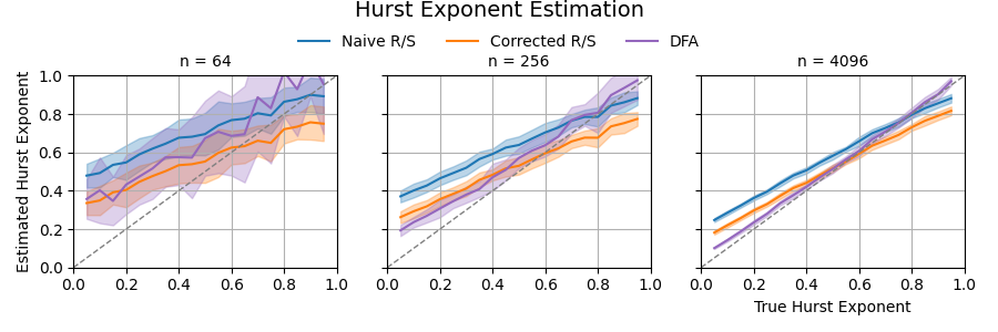
All four methods produce consistent estimates on synthetic fBm data. In practical applications to financial time series, DFA often performs best due to its robustness to non-stationarities and slow trends. In simulation studies where the true (H) is known, DFA consistently produces the most stable and accurate estimates.

The figure below illustrates the performance of these methods in simulation. For each method, we estimate the Hurst exponent across a range of ground truth values, using 100 trials of synthetic fBm per value. Each subplot corresponds to a different sample size ((n = 64, 512, 4096)). The shaded regions indicate one standard deviation around the mean estimate.

The code below computes the Hurst exponent using the Detrended Fluctuation Analysis method:

def hurst_dfa(x, min_window=4, max_window=None):
    if max_window is None:
        max_window = len(x) // 4

    x = np.cumsum(x - np.mean(x))
    window_sizes = []
    flucts = []

    n = min_window
    while n <= max_window:
        num_windows = len(x) // n
        if num_windows < 2:
            break

        reshaped = x[:num_windows * n].reshape(num_windows, n)
        x_vals = np.arange(n)
        # Fit and subtract trend for each window separately
        detrended = np.empty_like(reshaped)
        for i in range(num_windows):
            coeffs = np.polyfit(x_vals, reshaped[i], 1)
            trend = np.polyval(coeffs, x_vals)
            detrended[i] = reshaped[i] - trend

        fluct = np.sqrt(np.mean(detrended ** 2))
        window_sizes.append(n)
        flucts.append(fluct)
        n *= 2

    window_sizes = np.array(window_sizes)
    flucts = np.array(flucts)
    H = np.polyfit(np.log(window_sizes), np.log(flucts), 1)[0]
    return H

Applying fBm to Real Financial Series

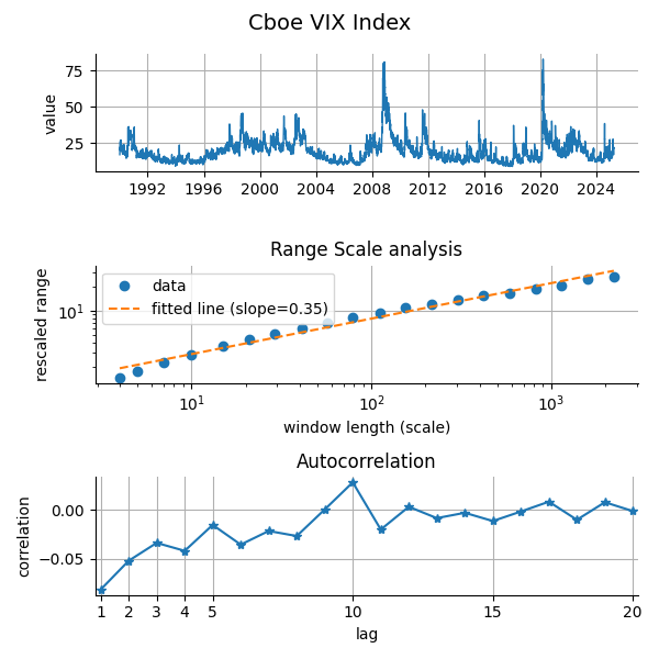
We now examine empirical time series through the lens of fBm. For the CBOE VIX index, the range-scale plot yields a slope of , indicating anti-persistence. The autocorrelation plot further supports this with mostly negative values.

This finding is consistent with the idea of rough volatility, as captured in the rough Bergomi model, which assumes that volatility follows a fractional process with a Hurst exponent significantly below 0.5.

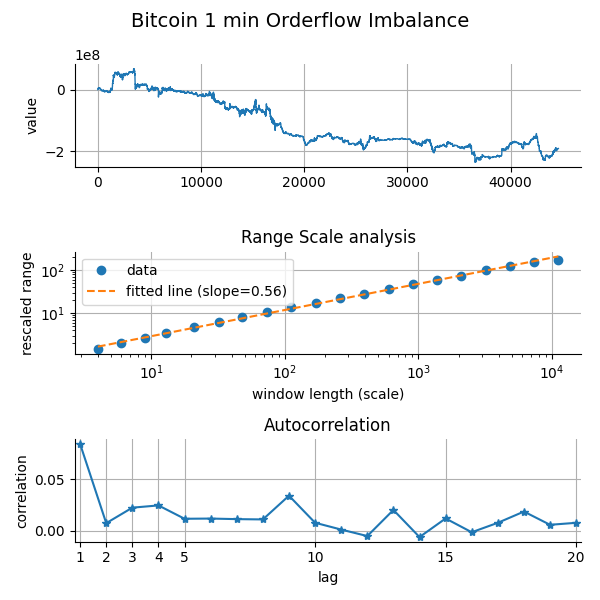
For high-frequency order flow imbalance (OFI) in Bitcoin, the behavior is different: here the estimated , suggesting mild persistence in the imbalance process.

To construct this time series, we used individual trade-level data from Deribit Bitcoin futures, and binned the trades into 1-minute intervals. Within each bin, we approximated the OFI by aggregating signed trade volumes, where buys add to the total and sells subtract from it. The resulting signal captures the net demand pressure within each interval.

Order Flow Imbalance is widely used in market microstructure research and by quantitative traders to detect short-term momentum or pressure. A consistently positive OFI indicates that market participants are predominantly buying, potentially driving the price upward, while a negative OFI signals net selling pressure. It’s a key variable in order book models, market impact estimation, and liquidity prediction, especially at intraday or tick-level resolutions.

The observation that OFI exhibits persistence suggests that supply-demand imbalances do not revert immediately but can last across several minutes. This aligns with the intuition that trading intentions, especially from larger participants, are executed over multiple slices or across multiple time bins.

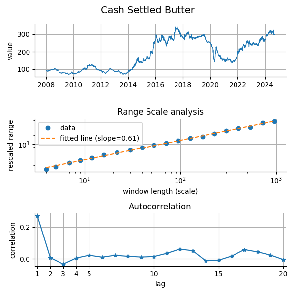
Finally, we consider a more obscure asset: the cash-settled butter futures market. This time, the estimated Hurst exponent is , indicating a relatively strong degree of persistence. In both the range-scale and autocorrelation diagnostics, the structure appears non-random and exhibits clear memory effects.

This result emerged from a broader scan we performed across 70 actively traded futures contracts, covering a diverse range of asset classes: equity indices, foreign exchange, interest rates, and commodities. While most contracts yielded Hurst exponents closer to the Brownian baseline or showed anti-persistent behavior, the butter futures stood out with its pronounced persistence.

This higher value suggests that deviations from the mean tend to persist longer and revert more slowly than in typical financial series. In practical terms, such behavior could reflect inventory-driven price trends or seasonal accumulation patterns that manifest in agricultural commodities. From a modeling perspective, this makes it an interesting candidate for applying memory-aware strategies, such as long-horizon trend filters or fractional volatility models.