Understanding the Uncertainty of Correlation Estimates – SITMO Machine Learning

Correlation is everywhere in finance. It’s the backbone of portfolio optimization, risk management, and models like the CAPM. The idea is simple: mix assets that don’t move in sync, and you can reduce risk without sacrificing too much return. But there’s a problem—correlation is usually taken at face value, even though it’s often some form of an estimate based on historical data. …and that estimate comes with uncertainty!

This matters because small errors in correlation can throw off portfolio models. If you overestimate diversification, your portfolio might be riskier than expected. If you underestimate it, you could miss out on returns. In models like the CAPM, where correlation helps determine expected returns, bad estimates can lead to bad decisions.

Despite this, some asset managers don’t give much thought to how unstable correlation estimates can be. In this post, we’ll dig into the uncertainty behind empirical correlation, and how to quantify it.

Consider the two sets of 20 random samples, the orange and green dots in Fig 1 below. In finance this could perhaps be the returns of two tech stocks over the last 20 weeks.

Each set is drawn from pairs of variables with the same true correlation $\rho=0.7$ . Even though both samples share the same underlying true correlation, the observed correlations from the samples differs. The left set of samples has a sample correlation of $r=0.66$ whereas the right has $r=0.43$ .

Fig 1. Two set of 20 2d random samples. Both sets of samples are drawn from a bivariate Normal distribution with the same correlation 0.7

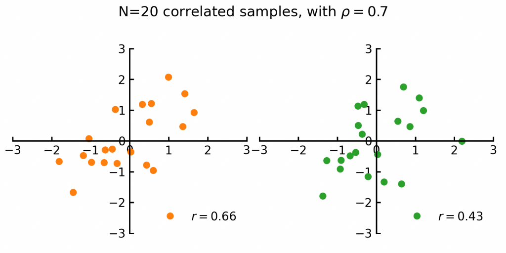
This illustrates the main issue: the observed correlation between random variables will never exactly match the true correlation, this is because we have a limited number of samples data.

The Correlation Sampling Distribution

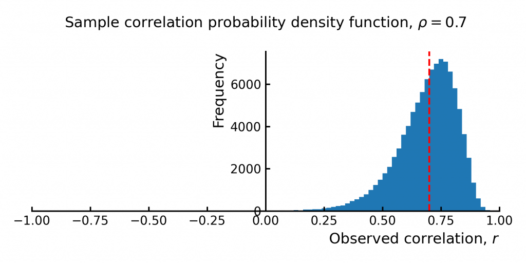
If we repeat this sampling many times -every time draw 20 correlated samples from two variables and then compute the observed correlation we get a distribution of possible sample correlations (Figure 2). This distribution shows the likelihood of observing different correlation values. Notice how the true correlation (red dashed line) sits centrally but the observed / computed correlations do not perfectly match the true correlation.

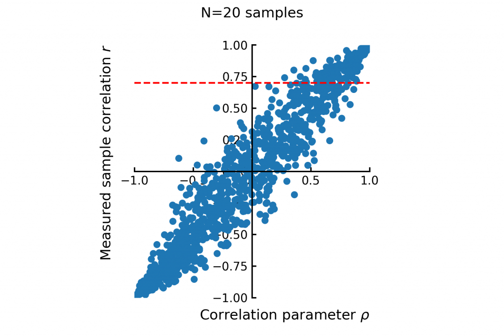
Fig 2. The distribution of computed sample correlation when we compute correlations based on 20 samples.

Expanding this concept further we can do this for a wide range of true correlations and then compare how the true and observed correlation relate. Figure 3 illustrates how sample correlations vary systematically with the true underlying correlation .

With this distribution we can answer questions like “if I observe a correlation of $\rho=0.7$ , what would the true correlation likely be?”. The answer to that question would be conditional distribution where $r=0.7$ , a slice throught the distribution along the red dotted line.

Fig 3. Distribution of true- vs estimated sample correlation.

It turns out this distribution has an analytical solution. The probability density function (pdf) of the sample correlation coefficient $r$ given the true correlation $\rho$ and sample size $N$ is known as Fisher’s exact formula for the sampling distribution of the correlation coefficient:

$\begin{align*}f(r) &= \frac{(N - 2) \Gamma(N - 1) (1 - \rho^2)^{\frac{N - 1}{2}} (1 - r^2)^{\frac{N - 4}{2}}}{\sqrt{2\pi} \Gamma(N - \frac{1}{2}) (1 - \rho r)^{N - \frac{3}{2}}} \\&\times {}_2F_1\left(\frac{1}{2}, \frac{1}{2}; N - \frac{1}{2}; \frac{\rho r + 1}{2}\right)\end{align*}$

where $\Gamma$ is the gamma function and ${}_2F_1$ is the Gaussian hypergeometric function.

The corresponding Python implementation is:

import numpy as np
from scipy.special import gammaln, hyp2f1

def correlation_confidence_pdf(N, rho, r):
    """
    Computes the probability density function (PDF) of the sample correlation coefficient.

    Parameters:
    - N: Sample size.
    - rho: correlation parameter.
    - r: Observed sample correlation coefficient.

    Returns:
    - PDF value at r.
    """
    # Compute logarithms of gamma functions for stability
    log_gamma_N_minus_1 = gammaln(N - 1)
    log_gamma_N_minus_half = gammaln(N - 0.5)

    # Compute the logarithm of the coefficient
    log_coeff = (
        np.log(N - 2)
        + log_gamma_N_minus_1
        + ((N - 1) / 2) * np.log(1 - rho**2)
        + ((N - 4) / 2) * np.log(1 - r**2)
        - 0.5 * np.log(2 * np.pi)
        - log_gamma_N_minus_half
        - (N - 1.5) * np.log(1 - rho * r)
    )

    # Compute the hypergeometric function
    hypergeom = hyp2f1(0.5, 0.5, N - 0.5, (rho * r + 1) / 2)

    # Combine the terms
    pdf = np.exp(log_coeff) * hypergeom

    return pdf

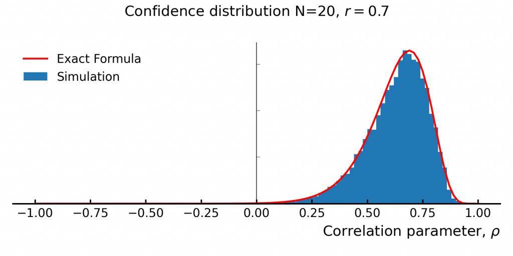
Figure 4 compares the exact formula against to simulation results (the slice in Fig 3).

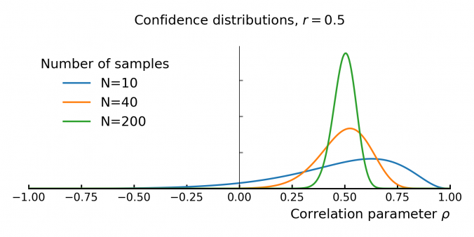
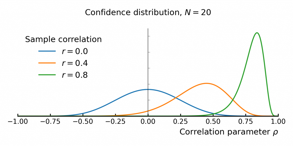
Fig 4. The Fisher exact formula vs the empirical simulated distribution.

The size of the dataset (N) significantly affects uncertainty: a larger number of samples lead to more precise correlation estimates (Figure 5). With fewer observations, the confidence distribution widens.

Fig 5. The impact of number of samples on the variance of the confidence distribution.

Similarly, uncertainty varies depending on the measured correlation itself. Estimates closer to zero have greater uncertainty, while values close to ±1 become more precise (Figure 6).

Fig 6. The impact of the observer correlation value on the confidence distribution of the true correlation.

Correlation Confidence Intervals

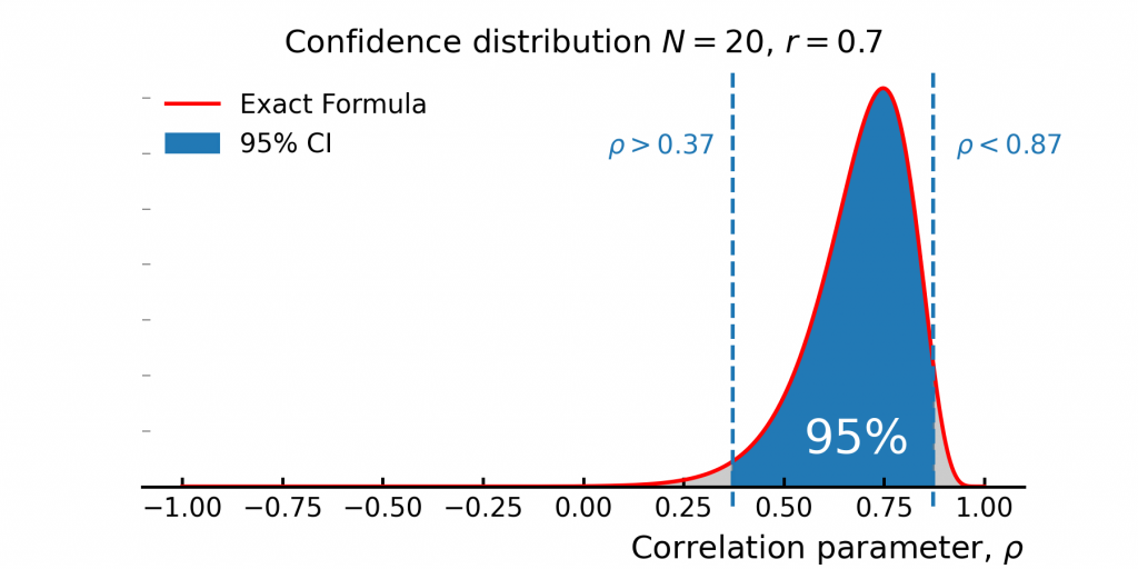
Now that we have the sampling distribution of the correlation coefficient, a common question is: “What range do we expect the true correlation to be in?” The distribution clearly has a central region where most of the probability is concentrated, but in theory, the true correlation could take on any value between -1 and +1.

Because of this, we refine the question slightly: “What’s the range in which we expect the true correlation to fall 95% of the time?” This is known as the 95% confidence interval (CI), illustrated in Figure 7. We define this range by cutting off the leftmost and rightmost 2.5% of the distribution, leaving the central 95%. In this example, the confidence interval extends from 0.37 to 0.87, giving us a practical estimate of where the true correlation is most likely to be.

Fig 7. The 95% confidence interval of the true correlation

One way to compute confidence intervals is by inverting the cumulative distribution function. However, for this distribution, that’s not practical -it doesn’t have a simple closed-form solution.

Fortunately, Fisher came up with a clever workaround. He introduced a transformation, now known as the Fisher transformation, which converts the sample correlation rrr into a variable that follows a more normally distributed shape. This makes it much easier to compute confidence intervals. The transformed value is:

$z = \frac{1}{2} \ln \left(\frac{1 + r}{1 - r}\right)$

The standard error of this transformed variable is:

$\sigma_z = \frac{1}{\sqrt{N - 3}}$

Using this, we can compute confidence bounds in Fisher’s Z-space:

$z_{\text{upper}} = z \pm z_{\alpha/2} \cdot \sigma_z$

where $z_{\alpha/2}$ is the critical value from the normal distribution (e.g., 1.96 for a 95% confidence level). Finally, we convert the bounds back to correlation space:

$\begin{align*}r_{\text{upper}} &= \frac{e^{2 z_{\text{upper}}} - 1}{e^{2 z_{\text{upper}}} + 1} \\r_{\text{lower}} &= \frac{e^{2 z_{\text{lower}}} - 1}{e^{2 z_{\text{lower}}} + 1}\end{align*}$

import numpy as np
from scipy.stats import norm

def correlation_confidence_interval(N, r, ci=0.95):
    """
    Computes the confidence interval for a sample correlation coefficient using Fisher's transformation.

    Parameters:
    - N: Sample size
    - r: Observed correlation coefficient
    - ci: Confidence level (default is 0.95 for a 95% confidence interval)

    Returns:
    - r_lower: Lower bound of the confidence interval
    - r_upper: Upper bound of the confidence interval
    """
    # Compute the significance level (alpha)
    alpha = 1.0 - ci

    # Apply Fisher's Z-transformation to the correlation coefficient
    z = 0.5 * np.log((1.0 + r) / (1.0 - r))

    # Compute the standard error of z and the corresponding margin of error
    dz = norm.ppf(1.0 - alpha / 2.0) * (1.0 / (N - 3.0))**0.5

    # Compute upper and lower bounds in Fisher's Z-space
    z_upper = z + dz
    z_lower = z - dz

    # Convert back from Fisher's Z-space to the correlation coefficient space
    r_upper = (np.exp(2.0 * z_upper) - 1.0) / (np.exp(2.0 * z_upper) + 1.0)
    r_lower = (np.exp(2.0 * z_lower) - 1.0) / (np.exp(2.0 * z_lower) + 1.0)

    return r_lower, r_upper

Hypothesis Test

Hypothesis Test: Is the Correlation Real?

So far, we’ve looked at confidence intervals, which tell us the likely range of the true correlation. But sometimes, we want to answer a different question: “Is the correlation strong enough to conclude that it’s real, or could it just be noise?”

Since any sample correlation comes with uncertainty, we need a way to test whether an observed $r$ is meaningfully different from zero. This is where hypothesis testing comes in. By checking how likely it is to observe a correlation as extreme as ours under the assumption that the true correlation is zero, we can decide whether to treat it as statistically significant.

Null hypothesis ( $H0$ ): The true correlation is $\rho = 0$ .
Alternative hypothesis ( $HA$ ): The true correlation is $\rho \neq 0$ .

To test this, we use the t-distribution, computing a test statistic:

$t = \frac{r \sqrt{N - 2}}{\sqrt{1 - r^2}}$

This follows a t-distribution with $N−2$ degrees of freedom. We compute a p-value based on this statistic, and if the p-value is small (typically <0.05), we reject the null hypothesis in favor of the alternative.

The following Python function implements this test:

from scipy.stats import t

def correlation_test_nonzero(N, r):
    """
    Performs a two-tailed t-test to assess if the correlation is significantly different from zero.

    Parameters:
    - N: Sample size
    - r: Observed correlation coefficient

    Returns:
    - probability: The probability that the correlation is nonzero (1 - p-value)
    """
    # Degrees of freedom
    df = N - 2

    # Compute t-statistic
    t_stat = r * np.sqrt(df) / np.sqrt(1 - r**2)

    # Compute two-tailed p-value
    p_value = 2 * (1 - t.cdf(abs(t_stat), df))

    # Return probability that correlation is nonzero
    return 1 - p_value

This test is widely used in finance when evaluating relationships between asset returns, factor models, and hedging strategies.

May your models converge and your residuals behave!