The Visible Shape of Random Galaxies: What You Get When You Project a 3D Disk – SITMO Machine Learning

When we look at galaxies through a telescope, we see them as ellipses. But real galaxies are 3D disks randomly oriented in space. This post shows how we can simulate that: we start with a random orientation, project a flat disk into the 2D image plane, and extract the observed ellipse parameters. This setup helps us understand what shape distributions we expect to see in the absence of structures like gravitational lensing and clustering.

In research we can analyse and compare the properties of this pure random reference model against real observations to look for subtle distortions

Random Galaxy Orientations in 3D

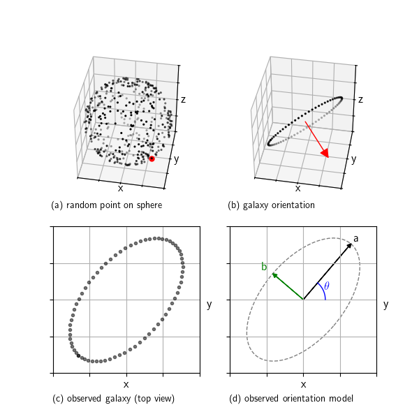
The top-left panel of the image shows points randomly distributed over a sphere. These represent random galaxy orientations, specifically, the normal vector to the galaxy’s disk. To generate these uniformly, we rely on a neat property of the multivariate Gaussian:

def random_3d_vectors(num_samples=1):
    """
    This works because the multivariate Gaussian is spherical symmetric, it looks the same in every direction.
    """
    p = np.random.normal(size=(num_samples, 3))
    p /= np.linalg.norm(p, axis=1, keepdims=True)
    return p

The idea is simple: the 3D normal distribution is spherically symmetric, so when we normalize 3 random Gaussian coordinates (x,y,z) to unit length and its direction is uniformly distributed over the sphere. This trick works with any spherically symmetric distribution, for instance, uniform inside a ball. But it doesn’t work with something like a unit cube, since a cube isn’t spherically symmetric.

Building a Disk from Its Normal Vector

To visualize the galaxy as a disk (or a flat circle), we need to construct a local coordinate frame lying in the galactic plane. This is done by creating two orthonormal vectors that lie perpendicular to the given normal vector. The result is a complete orthonormal basis: one vector is the normal, and the other two define the galaxy’s plane.

Here’s the code that constructs this basis:

def orthonormal_basis_from_normal(normals):
    """
    Given an (N, 3) array of 3D normal vectors, return two (N, 3) arrays,
    each representing a vector orthogonal to the input vector and to each other.
    """
    normals = np.asarray(normals)
    assert normals.shape[1] == 3

    N = normals.shape[0]
    u = np.zeros_like(normals)
    v = np.zeros_like(normals)

    ref = np.tile(np.array([0.0, 0.0, 1.0]), (N, 1))
    nearly_parallel = np.abs(np.sum(normals * ref, axis=1)) > 0.99
    ref[nearly_parallel] = np.array([1.0, 0.0, 0.0])

    u = np.cross(normals, ref)
    u /= np.linalg.norm(u, axis=1)[:, np.newaxis]

    v = np.cross(normals, u)
    v /= np.linalg.norm(v, axis=1)[:, np.newaxis]

    return u, v

What’s happening here is pure high school geometry. The cross product of the normal vector and any non-parallel reference vector gives a perpendicular vector $u$ in the plane. Then, taking the cross product of $n$ and $u$ gives a
second perpendicular vector $v$ , also lying in the plane. These two vectors $u$ and $v$ form the local galaxy plane basis.

Projecting the Galaxy Disk Into the Image Plane

We now place a circular disk in the galactic plane (spanned by $u$ and $v$ ) and
project it as seen from the observer. What we see is an ellipse, the top-down view
shown in the bottom-left panel. This is what you would actually observe in an image.

Extracting Ellipse Parameters From the Normal Vector

We can go a step further and directly compute the ellipse’s shape from the 3D normal vector, without projecting the full disk. The projected shape is always an ellipse, with a major axis $a$ , a minor axis $b$ , and an orientation angle $\theta$ . These can be derived using simple geometry:

$\begin{align*}a &= R \\b &= R |\cos \phi| = R |n_z| \\\theta &= \arctan2(n_y, n_x) + \frac{\pi}{2} \quad \text{(mod } 2\pi)\end{align*}$

Where $R$ is the true radius of the galaxy disk and $\vec{n} = (n_x, n_y, n_z)$ is
the unit normal vector. Here’s the corresponding code:

def ellipse_parameters_from_normals(normals, radius=1.0):
    """
    Given an (N, 3) matrix of normal vectors, compute the ellipse parameters (a, b, angle) for each.
    The angle is returned in radians, in the range [0, 2π), measured from the x-axis to the major axis.
    """
    normals = np.asarray(normals)
    normals = normals / np.linalg.norm(normals, axis=1, keepdims=True)

    nx, ny, nz = normals[:, 0], normals[:, 1], normals[:, 2]

    a = np.full(normals.shape[0], radius)
    b = radius * np.abs(nz)
    angle = np.arctan2(ny, nx) + np.pi / 2

    angle = np.mod(angle, 2 * np.pi)
    return a, b, angle

The angle is measured with respect to the $x$ -axis, and we add $\pi/2$ because
the direction of the major axis lies perpendicular to the projection of the normal.

What Should the Distribution Look Like?

If galaxy orientations are truly random in 3D, the observed shapes (as 2D ellipses)
follow a predictable statistical pattern. The next plot shows the histogram of
two quantities computed from 100.000 simulated galaxies:

The axis ratio $b/a$
The orientation angle $\Theta$

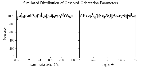
Both are uniformly distributed!

Any value of angle is equally likely, and all axis ratios between $0$ and $1$ occur with equal frequency. This is the baseline you’d expect without lensing or selection effects.

With this result we have a clean statistical benchmark for how galaxies should appear in a random universe, a handy model for detecting subtle deviations in
real observations.