Forecasting Current Market Turbulence with the GJR-GARCH Model – SITMO Machine Learning

The Current Market Shake-Up

Last week, global stock markets faced a sharp and sudden correction. The S&P 500 dropped 10% in just two trading days, its worst weekly since the Covid crash 5 years ago.

Big drops like this remind us that market volatility isn’t random, it tends to stick around once it starts. When markets fall sharply, that volatility often continues for days or even weeks. And importantly, negative returns usually lead to bigger increases in volatility than positive returns do. This behavior is called asymmetry, and it’s something that simple models don’t handle very well.

In this post, we’ll explore the Glosten-Jagannathan-Runkle GARCH model (GJR-GARCH), a widely-used asymmetric volatility model. We’ll apply it to real S&P 500 data, simulate future price and volatility scenarios, and interpret what it tells us about market expectations.

The GJR-GARCH Model

The GJR-GARCH model is part of a family of models developed to better understand how volatility behaves in financial markets.

The original ARCH model was introduced by Robert Engle in 1982. It was designed to solve a key weakness in models like Geometric Brownian Motion (GBM), which assume that volatility is constant over time. In reality, volatility is heteroskedastic, it changes over time, often clustering during periods of market stress.

Tim Bollerslev extended this idea with the GARCH model (Generalized ARCH) in 1986. The most widely used version is GARCH(1,1), which models volatility as a combination of three components:

A long-run average level of variance
The size of recent return shocks
The previous day’s variance

This allows volatility to evolve over time based on both recent market activity and past volatility, making it much more realistic than constant-volatility models.

However, GARCH(1,1) treats all return shocks the same way — whether the market moves up or down. This is a problem because real markets react more strongly to negative shocks. After a large loss, volatility tends to spike more than it would after a similarly sized gain. This is known as the leverage effect.

To address this, Glosten, Jagannathan, and Runkle introduced the GJR-GARCH model in 1993. It modifies the GARCH update equation by adding a term that activates only when returns are negative. This allows negative returns to have a greater impact on future volatility.

The GJR-GARCH model is defined as:

$\sigma_t^2 = \omega + \alpha \epsilon_{t-1}^2 + \gamma \cdot \mathbb{I}[\epsilon_{t-1} < 0] \cdot \epsilon_{t-1}^2 + \beta \sigma_{t-1}^2$

With:

$\epsilon_t$ is the return at time $t$ . These are typically daily log returns computed from historical price data.
$\sigma_t^2$ is the conditional variance, the model’s estimate of how volatile the return will be at time $t$ , based on all prior information.
$\omega$ is the baseline variance. It represents the long-run average level of variance when there are no recent shocks. This parameter must be strictly positive ( $\omega > 0$ ) to prevent the model from collapsing to zero volatility.
$\alpha$ controls how much recent return shocks influence today’s volatility. Specifically, it measures how sensitive the model is to the squared return from the previous day. This value should be non-negative ( $\alpha \geq 0$ ), since negative sensitivity doesn’t make sense in this context.
$\gamma$ captures the leverage effect, the additional impact of negative returns on volatility. When $\gamma > 0$ , the model responds more strongly to bad news (negative returns) than to good news. This term is also constrained to be non-negative ( $\gamma \geq 0$ ), so it doesn’t reduce volatility.
$\beta$ controls the persistence of volatility. A higher $\beta$ means that past volatility carries over more strongly into the present. This value must also be non-negative ( $\beta \geq 0$ ).

To keep the model well-behaved over time (stationary), we constrain the sum of the volatility feedback terms:

$\alpha + 0.5 \cdot \gamma + \beta \leq 1$

This condition ensures that the long-term (unconditional) variance of the process remains finite. If the sum is close to 1, volatility becomes very persistent and slow to revert. If it exceeds 1, the model becomes unstable, volatility can grow over time even in the absence of new shocks.

However, this version of the condition assumes that the model’s return shocks are symmetrically distributed, like in the standard normal noise we use below. For the more general cases, the correct stationarity condition is:

$\alpha + F(0) \cdot \gamma + \beta \leq 1$

Here, $F(0)$ is the probability that a return shock is negative, based on the distribution of the innovations (i.e., the CDF evaluated at zero). For symmetric distributions like the Gaussian, $F(0) = 0.5$ , which brings us back to the simplified version above. But for skewed or asymmetric innovations, this adjustment is necessary to correctly account for how often the leverage effect is activated.

Thanks to Simon Mauffrey @quantgestion.bsky.social for pointing out this important generalization.

The model is fit via maximum likelihood estimation. Assuming normally distributed innovations, the log-likelihood function is:

$\log L = -\frac{1}{2} \sum_{t=1}^T \left[ \log(2\pi \sigma_t^2) + \frac{(r_t - \mu)^2}{\sigma_t^2} \right]$

We minimize the negative average log-likelihood under parameter constraints to ensure stationarity and positivity.

Once the model is fitted, we simulate returns and volatility using the same update equation:

$\sigma_t^2 = \omega + (\alpha + \gamma \cdot \mathbb{I}[\epsilon_{t-1} < 0]) \cdot \epsilon_{t-1}^2 + \beta \cdot \sigma_{t-1}^2$

The return for each simulated time step is then:

$r_t = \mu + \epsilon_t, \quad \epsilon_t \sim N(0, \sigma_t^2)$

Getting the Data

To analyze recent market volatility, we use daily historical data for the S&P 500 index. This data can be downloaded directly from Nasdaq’s official website:

👉 Nasdaq S&P 500 Historical Data

We selected the “10-year” timeline to get a long enough sample for estimating a volatility model, and downloaded the data in CSV format. After saving the file as sp500.csv, we proceed to load and process it in Python.

The file contains daily prices with the most recent data at the top. We’ll sort it chronologically and compute backward-looking log returns, defined mathematically as:

$r_t = \log\left(\frac{P_t}{P_{t-1}}\right)$

This gives the percentage change from day ( t-1 ) to day ( t ), measured in continuous compounding terms (log scale). These returns serve as input to the volatility model.

Here’s how we load and compute the returns:

import pandas as pd
import numpy as np

# Load and sort historical S&P 500 data
data = pd.read_csv("sp500.csv", parse_dates=['Date'], index_col='Date')
data = data.sort_index()

# Compute backward-looking log returns
data['r'] = np.log(data['Close/Last'] / data['Close/Last'].shift(1))
data.dropna(inplace=True)

Defining the GJR-GARCH Model in Python

Here’s a complete implementation of the GJR-GARCH model in Python. It supports maximum likelihood estimation and forward simulation:

import numpy as np
from scipy.optimize import minimize, LinearConstraint, Bounds

class GJRGARCHModel:
    def __init__(self):
        # Model parameters, set after fitting
        self.mu = self.omega = self.alpha = self.gamma = self.beta = self.var0 = None
        self._eps = 1e-8  # Numerical lower bound to prevent division by zero
        self._fitted_variance = None  # Stores full variance sequence after fit
        self._fitted_residuals = None  # Stores residuals (returns - mu) after fit

    def __str__(self):
        # Pretty-print the model parameters
        if None in (self.mu, self.omega, self.alpha, self.gamma, self.beta, self.var0):
            return "GRJGARCHModel(not fitted)"
        return (
            f"GRJGARCHModel(\n"
            f"  mu={self.mu:.6f},\n"
            f"  omega={self.omega:.6f},\n"
            f"  alpha={self.alpha:.6f},\n"
            f"  gamma={self.gamma:.6f},\n"
            f"  beta={self.beta:.6f},\n"
            f"  var0={self.var0:.6f}\n"
            f")"
        )

    def _neg_log_likelihood(self, params, returns):
        """
        Compute the negative average log-likelihood of the GRJ-GARCH(1,1) model
        given a set of parameters and a return series.

        Parameters:
        - params: [mu, omega, alpha, gamma, beta, var0]
        - returns: array of returns

        Returns:
        - Negative mean log-likelihood (float)
        """
        mu, omega, alpha, gamma, beta, var0 = params

        # Reject invalid parameter values early
        if omega < self._eps or var0 < self._eps:
            return np.inf

        r = returns - mu             # residuals
        r2 = r**2                    # squared residuals
        is_negative = (r < 0).astype(float)  # indicator: 1 if return is negative, else 0
        T = len(r)

        var = np.empty(T)            # conditional variance sequence
        var[0] = max(var0, self._eps)

        # Recursively compute conditional variance
        for t in range(1, T):
            shock2 = r2[t - 1]
            var[t] = omega + (alpha + gamma * is_negative[t - 1]) * shock2 + beta * var[t - 1]
            if not np.isfinite(var[t]) or var[t] < self._eps:
                return np.inf

        var = np.maximum(var, self._eps)  # ensure numerical stability
        ll = -0.5 * (np.log(2 * np.pi * var) + r2 / var)
        return -np.mean(ll) if np.all(np.isfinite(ll)) else np.inf

    def fit(self, returns):
        """
        Fit the GRJ-GARCH model to a return series via maximum likelihood.

        Parameters:
        - returns: array of daily log returns

        Returns:
        - Optimization result from scipy.optimize.minimize
        """
        m, v = np.mean(returns), np.var(returns)  # empirical mean and variance
        x0 = np.array([m, v, 0.05, 0.05, 0.85, v])  # initial guess for parameters

        # Enforce positivity and stability
        bounds = Bounds(
            [-np.inf, self._eps, 0.0, 0.0, 0.0, self._eps],
            [ np.inf, np.inf,    1.0, 1.0, 1.0,  np.inf]
        )

        # Stationarity constraint: alpha + 0.5*gamma + beta <= 1
        constraint = LinearConstraint([[0, 0, 1, 0.5, 1, 0]], [0.0], [1.0])

        res = minimize(
            self._neg_log_likelihood, x0, args=(returns,),
            method='SLSQP', bounds=bounds, constraints=constraint
        )

        # Store optimal parameters
        self.mu, self.omega, self.alpha, self.gamma, self.beta, self.var0 = res.x

        # Compute and store residuals and variance sequence
        residuals = returns - self.mu
        r2 = residuals**2
        is_negative = (residuals < 0).astype(float)
        T = len(returns)

        var = np.empty(T)
        var[0] = max(self.var0, self._eps)
        for t in range(1, T):
            shock2 = r2[t - 1]
            var[t] = self.omega + (self.alpha + self.gamma * is_negative[t - 1]) * shock2 + self.beta * var[t - 1]

        self._fitted_variance = var
        self._fitted_residuals = residuals
        return res

    def sample(self, num_steps, num_paths, v0=None, random_state=None):
        """
        Simulate future returns and conditional variances from the fitted model.

        Parameters:
        - num_steps: number of time steps to simulate (e.g., 50 for 50 days)
        - num_paths: number of parallel paths to simulate
        - v0: initial variance value (float, array-like, or 'last' to use final fitted variance)
        - random_state: optional seed for reproducibility

        Returns:
        - returns: array of shape (num_paths, num_steps)
        - variance: array of shape (num_paths, num_steps)
        """
        if None in (self.mu, self.omega, self.alpha, self.gamma, self.beta, self.var0):
            raise RuntimeError("Model not fitted.")

        rng = np.random.default_rng(random_state)

        # Choose starting variance for all paths
        if v0 is None:
            init_var = np.full(num_paths, self.var0)
        elif v0 == 'last':
            if self._fitted_variance is None:
                raise ValueError("No fitted variance available. Call fit() first.")
            init_var = np.full(num_paths, self._fitted_variance[-1])
        else:
            init_var = np.broadcast_to(np.asarray(v0, dtype=float), (num_paths,))

        returns = np.zeros((num_paths, num_steps))
        variance = np.zeros_like(returns)
        var = np.maximum(init_var, self._eps)

        # Simulate shocks and update equations
        for t in range(num_steps):
            shock = rng.normal(0, np.sqrt(var))         # draw random shocks ~ N(0, var)
            returns[:, t] = self.mu + shock             # returns = mean + shock
            variance[:, t] = var                        # store current variance

            is_negative = (shock < 0).astype(float)
            var = self.omega + (self.alpha + self.gamma * is_negative) * shock**2 + self.beta * var

        return returns, variance

Fitting the Model

We now fit the model to the return series:

returns = data['r'].values
model = GJRGARCHModel()
model.fit(returns)
print(model)

This yields the following parameter estimates:

GJRGARCHModel(
  mu=0.000432,
  omega=0.000004,
  alpha=0.057259,
  gamma=0.214067,
  beta=0.806840,
  var0=0.000007
)

Interpretation:

mu = 0.000432: This is the model’s unconditional mean daily return. It’s small and positive, roughly 0.043% per day, consistent with long-term upward drift in equity markets.
omega = 0.000004: This is the long-run average variance. Its small value is typical, since daily returns have low absolute variance. It ensures volatility doesn’t collapse to zero when no shocks occur.
alpha = 0.057259: This parameter measures the immediate effect of any squared shock on volatility. Its magnitude suggests that volatility is moderately sensitive to recent innovations.
gamma = 0.214067: This is the key asymmetric term. The relatively high value here means negative shocks increase volatility much more than positive ones, confirming a pronounced leverage effect in the data.
beta = 0.806840: This is the persistence term. It shows that volatility depends heavily on its own past, a common feature in financial markets. Combined with alpha and gamma, it ensures slow decay of volatility spikes.
var0 = 0.000007: This is the initial conditional variance used at the start of the recursion. It has no interpretive meaning but is important for numerical stability.

This model-fit confirms that volatility is persistent and asymmetric, with negative returns having a stronger influence.

Making Forecasts

The two figures below show the output of the fitted GJR-GARCH(1,1) model: one for volatility, and one for price. Each line represents a single simulated future scenario, and the shaded area on the right shows the distribution of outcomes at the end of the forecast period.

Volatility Forecast

The first figure shows the evolution of annualized conditional volatility. The red line represents the historical volatility estimated by the model, and the faint blue lines are forward simulations. These represent what the model believes could happen to volatility in the near future, based on the current state of the market.

Volatility here refers to the model’s estimate of $\sigma_t$ , the standard deviation of returns at time $t$ . We annualize the conditional variance using the formula:

$\text{Annualized Volatility} = \sqrt{252 \cdot \sigma_t^2}$

In code, this looks like:

vol = np.sqrt(252 * var)

Since the model gives us $\sigma_t^2$ (variance), this conversion allows us to compare it with commonly reported annual volatility levels (e.g., 20% annual vol).

The KDE on the right shows the distribution of volatility at the forecast horizon, a summary of where volatility is likely to end up. In this case, although volatility spikes initially, the average scenario shows it gradually declining.

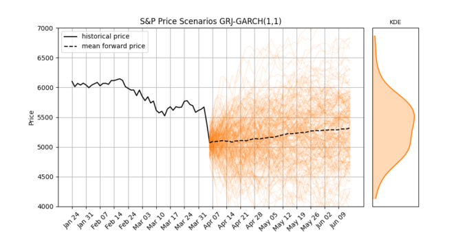
Price Forecast

The second figure shows simulated S&P 500 price paths over the same period. The black line represents the historical index level. The orange lines are future simulations, each built by compounding the model’s simulated returns forward from the last observed price. The mean of all paths is shown with a dashed black line.

The KDE on the right displays the distribution of prices at the final forecast date. This gives us a view of the range of potential outcomes implied by the model, both in terms of upside and downside risk.

Wrap up

Models like GARCH and GJR-GARCH aren’t just useful for visualizing volatility, they’re powerful tools for risk management, scenario analysis, and derivatives pricing.

Once fitted, they can be used to estimate Value-at-Risk (VaR), compute the probability of large drawdowns, or generate volatility surfaces for option models. They also form the core of many real-world trading and hedging systems. While they don’t predict the future, they help quantify what kinds of futures are possible, and how likely they are