A Tiling That Never Repeats – SITMO Machine Learning

This image below shows a tiling made from just two simple shapes, arranged in a pattern that never repeats. You can extend it as far as you like, and it will keep growing in complexity without ever falling into a regular cycle. That property alone makes it interesting, but the background is even better.

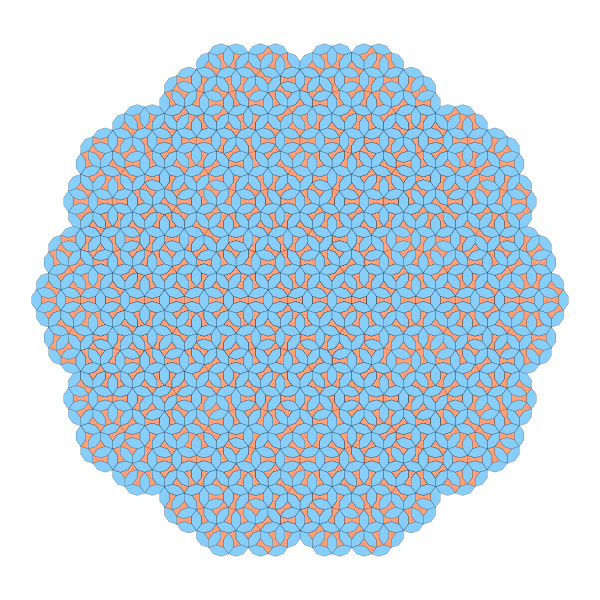
Most of the tilings we come across use shapes like squares or hexagons. These rely on 3-, 4-, or 6-fold symmetry and produce patterns that repeat periodically. But the tiling above is built on 5-fold symmetry, which cannot fill the plane in a repeating way. That’s what gives it this intricate, non-repeating structure.

I first came across this type of pattern during the Dutch National Science Quiz in 2014 (which, incidentally, we won! (and we won again a 2nd time later)). One of the questions was about this tiling. At the time, I had no idea how deep the math behind it went. Later I learned about the work of Roger Penrose, who studied these so-called aperiodic tilings and helped explain why such patterns behave the way they do.

Even more surprising is that similar patterns were already being used in Islamic architecture over 800 years ago. A set of five tiles, now referred to as “girih tiles”, was used by artisans to decorate mosques and madrasas across the Islamic world. These designs turn out to encode mathematical structures that weren’t formally studied until the 20th century. It appears that artisans used the tiles as practical tools to construct highly regular, yet non-repeating, patterns, without necessarily having a formal theory of aperiodicity. The intuition and craftsmanship involved is remarkable.

The Two Shapes: Shesh Band and Sormeh Dan

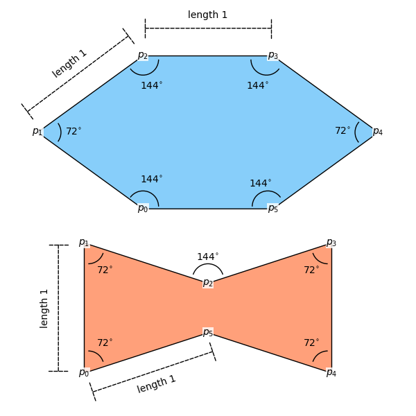
To build the tiling, we’ll use just two shapes. Both come from the tradition of girih tiles in Islamic art and are known by their Persian names: the Shesh Band, which means “six strap” and is an elongated hexagon, and the Sormeh Dan, a bow tie–like shape. You can spot them both in the full tiling above, often arranged in tight interlocking patterns.

What’s special about these shapes is that they are built entirely from angles related to 5-fold symmetry. The main angle is 72°, which comes from dividing a circle into five equal parts (360° / 5). The other angles that show up — 144°, 36°, and 18° — are all derived from that. In fact, every corner in both shapes is either 72° or 144°, and that restriction plays a key role in why the tiling avoids repetition.

Another important detail is that all edges have the same length. This is what allows the shapes to fit together edge-to-edge without gaps, and it’s what lets us construct them cleanly using basic trigonometry.

Below is a plot of the angles and side lengths:

And here’s how we compute the vertex coordinates from trigonometry:

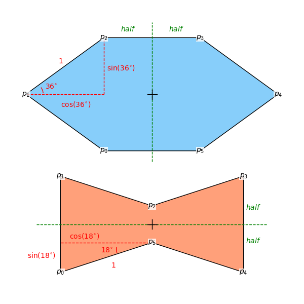
Both shapes are centered around the origin and defined in local coordinates, using sine and cosine of 18° and 36°, which are the key internal angles. The following code builds both polygons as NumPy arrays. We’ll use them later as base shapes for all our transformations.

# Core angles and trigonometric constants
half = 0.5
angle = np.pi / 10  # 18 degrees
sa, ca = np.sin(angle), np.cos(angle)
sb, cb = np.sin(2 * angle), np.cos(2 * angle)

# Golden ratio and scale
phi = (1 + np.sqrt(5)) / 2
scale_factor = phi**-2

# Base polygon definitions (in local coordinates)
base_tie_shape = np.array([
    (-ca, -half),
    (-ca,  half),
    (  0,  half - sa),
    ( ca,  half),
    ( ca, -half),
    (  0, -half + sa)
])

base_hex_shape = np.array([
    (-half,    -sb),
    (-half - cb, 0),
    (-half,     sb),
    ( half,     sb),
    ( half + cb, 0),
    ( half,    -sb)
])

Positioning Tiles with Transformations

To build up a complex tiling from a few basic shapes, we need a way to position those shapes in the right place and orientation. This means applying geometric transformations like rotation, scaling, and translation to our base polygons. Each tile in the pattern is just a transformed copy of either the bow tie or the hexagon.

This is a common topic in computer graphics and geometry, and there’s a standard mathematical tool that handles all these operations at once: the homogeneous transformation matrix.

A transformation in 2D that combines a rotation by an angle $\theta$ , a uniform scale by $s$ , and a translation by $(t_x, t_y)$ is written as a $3 \times 3$ matrix:

$T =\begin{bmatrix}s \cos\theta & -s \sin\theta & t_x \\s \sin\theta & s \cos\theta & t_y \\0 & 0 & 1\end{bmatrix}$

Each part of this matrix plays a specific role:

$s$ is a scaling factor that stretches or shrinks the shape.
$\theta$ is the rotation angle, measured counterclockwise in radians.
$t_x$ and $t_y$ are translation values that shift the shape along the x- and y-axes.
The third row $[0\ 0\ 1]$ is what enables translation to be written as a matrix multiplication, a trick made possible by working in homogeneous coordinates.

To apply this matrix, we represent each 2D point $(x, y)$ as a 3D vector $(x, y, 1)$ . This way, we can compute the transformed point using matrix multiplication, and all geometric operations (scaling, rotation, and translation) are applied together in one step.

If we want to apply multiple transformations in sequence -for example, rotate, then scale, then translate- we can combine them by multiplying the matrices:

$T_{\text{total}} = T_3 T_2 T_1$

Note that the last transformation in the list is applied first. This ordering may feel backward, but it mirrors how function composition works.

In this project, we associate each tile with a sequence of transformations. These transformations are stored as parameter tuples: (theta_degrees, scale, tx, ty). When a tile needs to be drawn, we convert this list into a single transformation matrix and apply it to the tile’s base shape.

Here’s the code that does that:

def compose_2d_transform(params):
    """
    Constructs a 3x3 homogeneous transformation matrix from rotation (degrees), 
    uniform scaling, and 2D translation.

    If a list of parameter tuples is provided, the transformations are composed 
    in the given order (last applied first).

    Parameters:
        params (tuple or list of tuples): Each tuple must contain:
            (theta_degrees, scale, tx, ty)

    Returns:
        np.ndarray: A 3x3 homogeneous transformation matrix.
    """
    if isinstance(params, list):
        transform = np.eye(3)
        for step in reversed(params):
            transform = transform @ compose_2d_transform(step)
        return transform

    theta_deg, scale, tx, ty = params
    theta_rad = np.deg2rad(theta_deg)
    cos_t, sin_t = np.cos(theta_rad), np.sin(theta_rad)

    linear_part = scale * np.array([[cos_t, -sin_t],
                                    [sin_t,  cos_t]])

    H = np.eye(3)
    H[:2, :2] = linear_part
    H[:2, 2] = [tx, ty]
    return H


def apply_2d_transform(points, transform):
    """
    Applies a homogeneous 2D transformation matrix to a set of points.

    Parameters:
        points (np.ndarray): An (n, 2) array of 2D points.
        transform (np.ndarray): A 3x3 homogeneous transformation matrix.

    Returns:
        np.ndarray: The transformed (n, 2) array of points.
    """
    n = points.shape[0]
    homog = np.hstack([points, np.ones((n, 1))])
    transformed = (transform @ homog.T).T
    return transformed[:, :2]

Substitution Rules

Now that we can position and transform individual tiles, we’re ready to talk about the core idea behind this tiling: substitution.

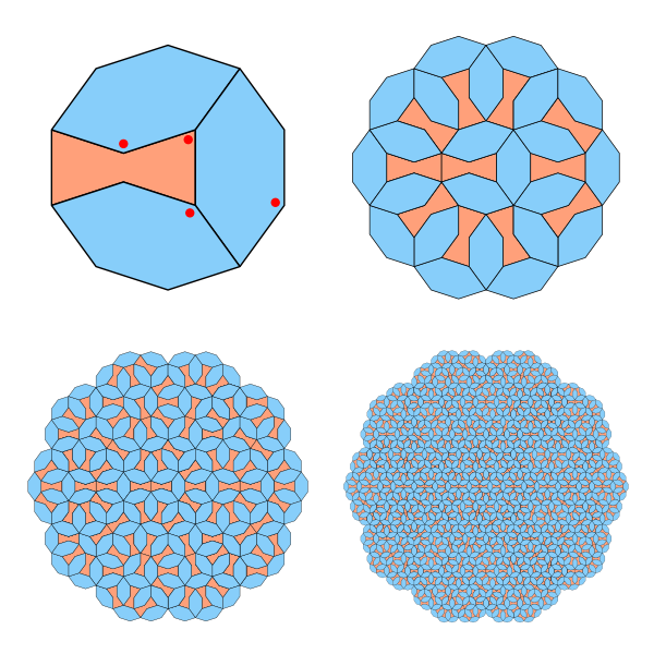
The method is recursive. We begin with a few tiles at a certain size and orientation. At each step, we replace every tile with a new configuration of smaller tiles, using a predefined pattern. These substitution patterns preserve the 5-fold symmetry, but they scale everything down and introduce more complexity. After repeating this a few times, the pattern starts to grow outward with an astonishing amount of structure, and it never repeats.

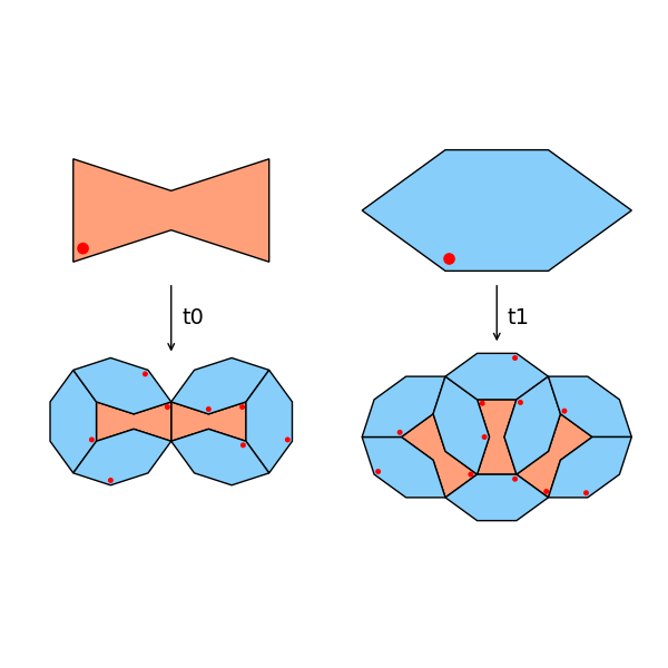
The top row shows the two shapes we’re working with: the bow tie (Sormeh Dan) on the left and the elongated hexagon (Shesh Band) on the right. A red dot is used to indicate the orientation of each tile, a visual cue that becomes important once we start rotating and flipping tiles.

Each substitution rule defines how to replace a single tile with a group of smaller tiles:

A bow tie is replaced using the rule we call t0, shown at the bottom left. The result is a set of two smaller bow ties and several hexagons. Notice how the two new bow ties are both rotated by 180°, flipping the original orientation.
A hexagon is replaced using the rule t1, shown at the bottom right. It creates a ring-like structure of hexagons and bow ties.

Orientation matters. These replacements are not applied blindly, they are transformations. The red dot shows how each tile keeps track of its own frame of reference, so that when it’s replaced, the new tiles are positioned and rotated relative to that frame.

The code below defines the two substitution rules, and how to apply them to a list of tiles. Each tile is represented as a list of transformations, which we compose into a single transformation matrix when it’s time to draw.

def make_t0():
    ties = [
        [(-180, 1, ca, 0)],
        [(-180, 1,-ca, 0)]
    ]

    hexs = [
        [(90, 1, -2*ca-sb, 0)],
        [(0,1) + tuple(*-base_hex_shape[[2]]), (-180 - 18, 1, -ca, half - sa)],
        [(0,1) + tuple(*-base_hex_shape[[0]]), (18, 1, ca, half - sa)],
        [(0,1) + tuple(*-base_hex_shape[[3]]), (90, 1, 2 * ca, half)],
        [(0,1) + tuple(*-base_hex_shape[[0]]), (-180 - 18, 1, 2 * ca, -half)],
        [(0,1) + tuple(*-base_hex_shape[[2]]), (18, 1, -2 * ca, -half)]

    ]
    # scale
    ties = [t + [(0,scale_factor,0,0)] for t in ties]
    hexs = [t + [(0,scale_factor,0,0)] for t in hexs]

    return ties, hexs


def apply_t0(ties):
    new_ties = []
    new_hexs = []

    t0_ties, t0_hexs = make_t0()

    for old_tie in ties:
        new_ties = new_ties + [ t0_tie + old_tie for t0_tie in t0_ties]
        new_hexs = new_hexs + [ t0_hex + old_tie for t0_hex in t0_hexs]
    return new_ties, new_hexs



def make_t1():
    ties = [
        [(0,1) + tuple(*-base_tie_shape[[0]]), (90+36, 1) + tuple(*base_hex_shape[[2]])],
        [(0,1) + tuple(*-base_tie_shape[[4]]), (-90, 1) + tuple(*base_hex_shape[[2]])],
        [(0,1) + tuple(*-base_tie_shape[[0]]), (90-36, 1) + tuple(*base_hex_shape[[4]])],

    ]

    hexs = [
        [(-180,1,0,0)],
        [(0,1) + tuple(*-base_hex_shape[[4]]), (-36, 1) + tuple(*base_hex_shape[[1]])],
        [(0,1) + tuple(*-base_hex_shape[[4]]), (36, 1) + tuple(*base_hex_shape[[1]]), (0,1,0,2*sb+2*ca)],
        [(0,1) + tuple(*-base_hex_shape[[1]]), (+90+18, 1) + tuple(*base_hex_shape[[2]])],
        [(-180,1,0,0), (0,1,0,2*sb+2*ca)],

        [(0,1) + tuple(*-base_hex_shape[[4]]), (-90-18, 1) + tuple(*base_hex_shape[[3]])],
        [(0,1) + tuple(*-base_hex_shape[[1]]), (-36, 1,0,0), (0,1,1/2+cb,2*sb+2*ca)],
        [(0,1) + tuple(*-base_hex_shape[[1]]), (36, 1) + tuple(*base_hex_shape[[4]])],

    ]
    # shift down
    ties = [t + [(0,1,0,-sb-ca)] for t in ties]
    hexs = [t + [(0,1,0,-sb-ca)] for t in hexs]
    # scale
    ties = [t + [(0,scale_factor,0,0)] for t in ties]
    hexs = [t + [(0,scale_factor,0,0)] for t in hexs]


    return ties, hexs


def apply_t1(hexs):
    new_ties = []
    new_hexs = []

    t0_ties, t0_hexs = make_t1()

    for old_hex in hexs:
        new_ties = new_ties + [ t0_tie + old_hex for t0_tie in t0_ties]
        new_hexs = new_hexs + [ t0_hex + old_hex for t0_hex in t0_hexs]
    return new_ties, new_hexs

Recursive Substitution

We now have all the ingredients: two shapes, a way to transform them, and substitution rules that expand each tile into a configuration of smaller ones. The last step is to actually run the recursive process.

We begin with a small initial configuration, shown in the top-left of the figure below. It’s a curved loop of four tiles, cut from the structure that appears in the t0 substitution. This gives us a compact starting point that already respects the symmetry and local matching rules.

The initial configuration is defined like this:

ties = [
    [(180,1,0,0)]
]

hexs = [
    [(0,1) + tuple(*-base_hex_shape[[1]]), (18,1) +  tuple(*base_tie_shape[[1]])],
    [(0,1) + tuple(*-base_hex_shape[[3]]), (90,1) +  tuple(*base_tie_shape[[3]])],
    [(0,1) + tuple(*-base_hex_shape[[0]]), (180-18,1) + tuple(*base_tie_shape[[4]])],
]

# shift to the right
dx = sb
ties = [t + [(0,1, -dx, 0)] for t in ties]
hexs = [t + [(0,1, -dx, 0)] for t in hexs]

From there, we apply our substitution rules recursively:

num_rounds = 4
for round in range(num_rounds):

    if round == num_rounds -1:
        break

    new_ties_0, new_hexs_0 = apply_t0(ties)
    new_ties_1, new_hexs_1 = apply_t1(hexs)
    ties = new_ties_0 + new_ties_1
    hexs = new_hexs_0 + new_hexs_1

which gives us the tiling at the top of this post!