Gravitational lensing is one of the most beautiful predictions of general relativity.
When a massive object, like a galaxy or black hole, lies between a distant light source and an observer, the gravitational field bends the path of light rays, distorting and duplicating the image of the background object. In this post, we’ll build a simple but realistic raytracer that simulates this phenomenon in two dimensions.
We’ll walk through the model, the equations, and the Python implementation. The result is a function that takes a 2D image and simulates how it would appear if viewed through a point-mass gravitational lens.
The Gravitational Lens Geometry
The figure below shows the standard gravitational lens setup (image source: Wikipedia):
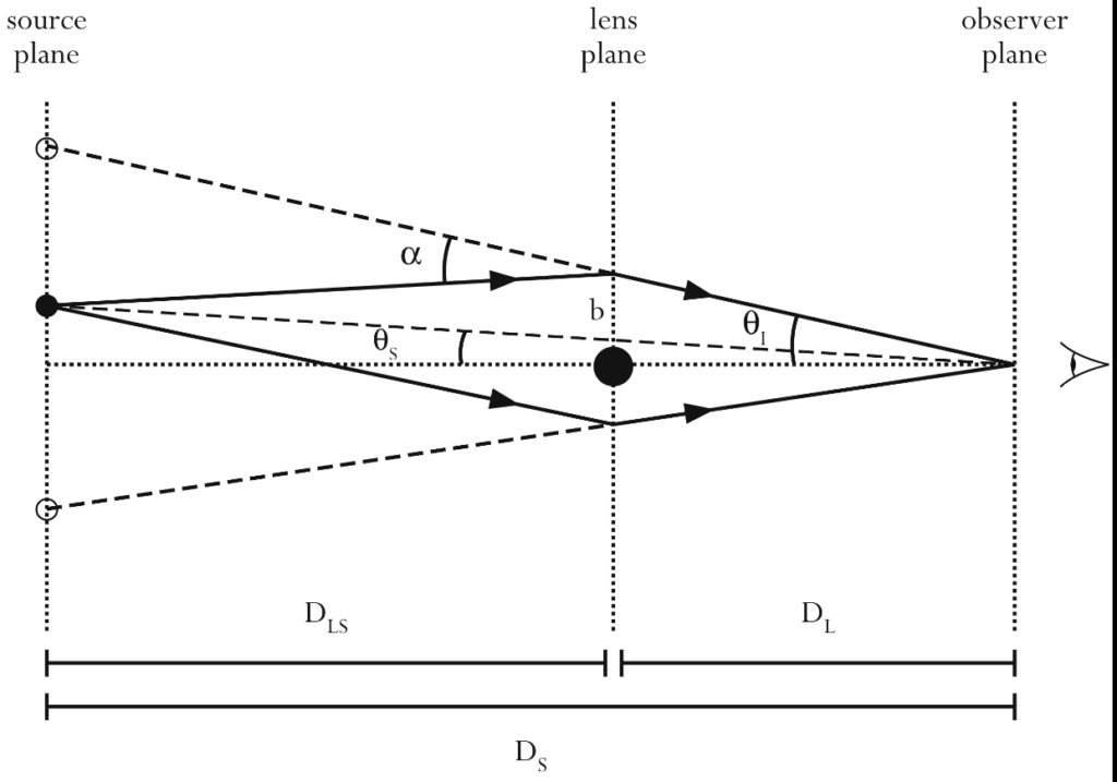
A background source (on the left) emits light rays that are bent by the gravitational field of the lens (middle), and reach the observer (right) from multiple paths. The key geometric quantities are:
 : distance from observer to source
 : distance from observer to lens
 : distance from lens to source
 : angle of the image as seen from the observer
 : angle of the true source position
 : total deflection angle
 : impact parameter (distance of the ray from the lens center in the lens plane)
In this model, we ignore light propagation time and use the thin-lens approximation. That is, we assume the bending happens in a single plane (the lens plane), and rays travel in straight lines on either side of it.
The Lens Equation
The central relation is the lens equation, which links the observed angle to the true source angle via the deflection angle:
![\[\theta_S = \theta_I - \alpha(\theta_I)\]](https://www.sitmo.com/wp-content/ql-cache/quicklatex.com-e67a39ca60181b7f4fc7e787d6c1f0d6_l3.png "Rendered by QuickLaTeX.com")
For a point mass lens, the deflection angle magnitude is given by:
![\[\alpha = \frac{4GM}{c^2} \cdot \frac{1}{b}\]](https://www.sitmo.com/wp-content/ql-cache/quicklatex.com-2f214c4d4bf59a34de0975cf35e4f018_l3.png "Rendered by QuickLaTeX.com")
The bending is stronger near the lens center, diverging as  . In our 2D simulation, we model this by applying a radial field that deflects each pixel depending on its distance from the lens.
Thin-Film Approximation
We implement the lensing effect using the thin film approximation, which is a
simplified, flat-space mapping. Instead of computing full geodesics in curved spacetime, we treat the lens as a static distortion field applied to an image plane. This captures strong lensing effects like double images and arcs, though it does not include time delay or shear from extended mass distributions.
The Raytracer Code
Here’s the Python implementation:
def gravitational_lens(image, lens_pos=(410, 420), C=2e5):
    h, w, _ = image.shape
    y, x = np.mgrid[0:h, 0:w]

    dx = x - lens_pos[0]
    dy = y - lens_pos[1]
    r = np.sqrt(dx**2 + dy**2)
    r_safe = np.where(r == 0, 1e-6, r)

    # Apply deflection field
    b = r - C / r_safe
    f = b / r_safe
    src_x = lens_pos[0] + dx * f
    src_y = lens_pos[1] + dy * f

    # Clip to image bounds
    src_x = np.clip(src_x, 0, w - 1)
    src_y = np.clip(src_y, 0, h - 1)

    # Sample RGB channels
    warped = np.zeros_like(image)
    for c in range(3):
        warped[:, :, c] = map_coordinates(image[:, :, c], [src_y.ravel(), src_x.ravel()], order=1).reshape(h, w)

    return warped
Details about the code
This function creates a raytraced view of the image as seen through a gravitational
lens at lens_pos, which is a 2D coordinate in pixel space. The constant C determines the strength of the lensing. Larger values cause stronger bending, mimicking more massive or closer lenses.
We compute the radial distance r from each pixel to the lens center, then apply the lensing formula:
![\[b = r - \frac{C}{r} \quad \text{and} \quad f = \frac{b}{r}\]](https://www.sitmo.com/wp-content/ql-cache/quicklatex.com-bb145d8f52dee322908d356e1b22829b_l3.png "Rendered by QuickLaTeX.com")
This gives a displacement factor f applied to the pixel vector (dx, dy). The
resulting coordinates (src_x, src_y) indicate where each pixel’s light originates from in the unlensed image.
We use scipy.ndimage.map_coordinates to sample the RGB values at those positions, performing bilinear interpolation to fill in the warped image.
Parameters
image: RGB NumPy array of shape(H, W, 3)lens_pos: location of the lens center in pixel coordinatesC: strength of the lensing field (proportional to lens mass and inverse distance)
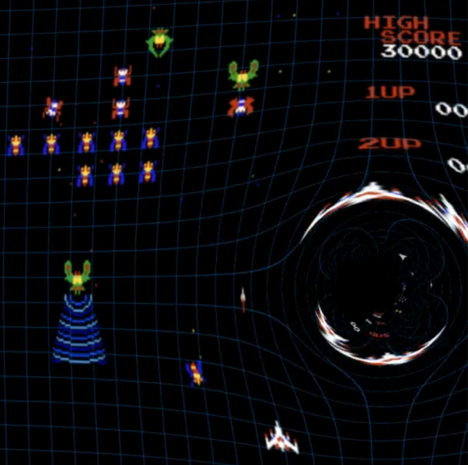
You can now animate this by moving the lens position like we did in the animation above!