Faster Monte Carlo Exotic Option Pricing with Low Discrepancy Sequences – SITMO Machine Learning

In this post, we discuss the usefulness of low-discrepancy sequences (LDS) in finance, particularly for option pricing. Unlike purely random sampling, LDS methods generate points that are more evenly distributed over the sample space. This uniformity reduces the gaps and clustering seen in standard Monte Carlo (MC) sampling and improves convergence in numerical integration problems.

A key measure of sampling quality is discrepancy, which quantifies how evenly a set of points covers the space. Low-discrepancy sequences minimize this discrepancy, leading to faster convergence in high-dimensional simulations.

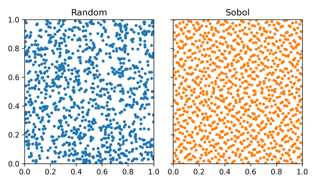
The difference between standard random sampling and low-discrepancy sequences can be seen in the plot below. On the left we see regular random sampling of a 2D square results in uneven clustering and gaps. On the right we see sampling using Sobol sequences that distribute points more evenly across the area.

A natural question is whether a regular grid would be the best way to achieve low discrepancy. In low dimensions, grids can indeed provide excellent coverage, but they become impractical as the number of dimensions increases. The Asian Basket option pricing example that we’ll explore below is a 60-dimensional problem (5 assets × 12 time points for averaging). Even if we were to place just 2 points per dimension, this would require $2^60 \approx 10^18$ samples, an astronomical number. This is why low-discrepancy sequences are used instead of grids: they provide structured, uniform coverage without requiring an exponentially growing number of points as a function of dimension.

Another key advantage of low-discrepancy sequences over grids is their incremental nature. A grid requires a fixed number of points in advance, making it rigid and impractical for many applications. In contrast, low-discrepancy sequences allow for progressive sampling—new points are always placed in the largest existing gaps, refining the coverage without requiring a full recomputation. This makes them especially useful for Monte Carlo-style simulations, where one can keep adding samples dynamically without needing to specify the total number upfront.

Convergence Rates: MC vs. QMC

The efficiency of these methods is often measured by their convergence rates. Standard MC methods typically exhibit a convergence rate proportional to $\frac{1}{\sqrt{N}}$ , where $N$ is the number of samples. This convergence rate comes from the Central Limit Theorem (CLT). In MC simulations, the estimated mean of a quantity (e.g., an option price) is an average of $N$ independent samples, and in that case the standard deviation of the sample mean decreases with the square root. This means that to reduce the error by a factor of 10, one must increase the number of samples by a factor of 100.

In contrast, QMC methods using low-discrepancy sequences aim for a convergence rate closer to $\frac{1}{N}$ . While this rate is not always guaranteed, in practice, QMC often achieves significantly faster convergence than standard MC methods. This improvement is due to the more uniform coverage of the sample space provided by low-discrepancy sequences.

Background on Low-Discrepancy Sequences

Low-discrepancy sequences are designed to cover a multi-dimensional space more uniformly than uncorrelated random points. Several types of LDS have been developed:

van der Corput Sequence: One of the earliest examples, focusing on one-dimensional distributions.
Halton Sequence: Extends the van der Corput sequence to higher dimensions using different prime bases for each dimension.
Hammersley Set: Similar to the Halton sequence but includes a linear sweep in one dimension, providing even distribution when the number of points is known in advance.
Sobol Sequence: Developed by Russian mathematician Ilya M. Sobol’ in 1967, this sequence is widely used due to its efficiency in high-dimensional integration problems.

Among these, the Sobol sequence has gained popularity, especially in financial applications. I think this is maily because there were some early papers and software libraries that made Sobol sequences easy to use. In terms of performance most LDS sequences will perform similar, there is not a strong preference.

Scrambled Sobol Sequences

Initially people found a couple of issues with Sobol where the data was not uniform and independent between dimensions. To overcome that are scrambling techniques was applied, which is nowadays a standard extension. Scrambling introduces better mixing while preserving the low-discrepancy characteristics, leading to better uniformity and improved convergence in practical applications. The scipy.stats.qmc module in SciPy provides an implementation of scrambled Sobol sequences.

Application to Asian Basket Option Pricing

To illustrate the practical benefits of QMC methods, we apply both MC and QMC to a somehwat typical toy problem, to price an Asian Basket option. This type of derivative has a payoff dependent on the arithmetic average of multiple correlated assets over time. Since this option depends on a time-average rather than a final price, and also on the weighted average of a basket of correlated assets, it does not have a simple closed-form solution. Instead, we use simulation-based methods.

The option’s payoff is:

$\text{Payoff} = \max\left(0, \frac{1}{T}\sum_{t=1}^{T} S_{\text{basket},t} - K\right)$

where the basket price at time tt is a weighted sum of asset prices:

$S_{\text{basket},t} = \sum_{i=1}^{N} w_i S_{i,t}$

To model the stock prices, we assume they follow a standard multivariate geometric Brownian motion (GBM), which accounts for correlation between assets:

$dS_i(t) = S_i(t)\left(r - \frac{1}{2}\sigma_i^2\right)dt + S_i(t)\sigma_i dW_i(t)$

where $\sigma_i$ is the volatility of asset $i$ , $r$ is the risk-free rate, and $dW_i$ represents correlated Brownian motion increments.

For those who prefer code over equations, the function simulate_paths below implements this process.

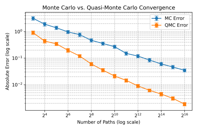
While there are sophisticated numerical approximantion methods for this type of option (see e.g. “Partially Exact and Bounded Approximations for Arithmetic Asian Options”, Roger Lord, 2005) our goal here is to illustrate the impact of using QMC vs. MC in pricing. We simulate asset paths, compute payoffs, and compare results across different sample sizes. The plot below shows how QMC significantly reduces pricing error compared to MC as the number of paths increases. Looking along a horeizontal line, we see that $2^9=512$ samples base QMC results is more accurate than the $2^16=65.536$ samples regular MC result with is more than 100x more expensive in terms of computing time.

Below is the Python implementation of the main equations above:

import numpy as np
import scipy.stats as stats
from scipy.linalg import cholesky
from scipy.stats.qmc import Sobol

def generate_standard_normal_mc(n_paths, n_steps, n_assets, seed=None):
    if seed is not None:
        np.random.seed(seed)
    return np.random.normal(size=(n_paths, n_steps, n_assets))

def generate_standard_normal_qmc(n_paths, n_steps, n_assets):
    sobol = Sobol(d=n_steps * n_assets, scramble=True)
    U = sobol.random(n=n_paths)
    return stats.norm.ppf(U).reshape(n_paths, n_steps, n_assets)

def simulate_paths(Z, S0, sigma, risk_free_rate, dt, correlation_matrix):
    n_paths, n_steps, n_assets = Z.shape
    L = cholesky(correlation_matrix, lower=True)
    dW = np.matmul(Z, L.T) * np.sqrt(dt)
    
    S = np.zeros((n_paths, n_steps + 1, n_assets))
    S[:, 0, :] = S0

    for t in range(1, n_steps + 1):
        S[:, t, :] = S[:, t-1, :] * np.exp((risk_free_rate - 0.5 * sigma**2) * dt + sigma * dW[:, t-1, :])
    
    return S

def compute_asian_basket_payoff(S, weights, strike, risk_free_rate, T):
    basket_prices = np.sum(S[:, 1:, :] * weights, axis=2)
    avg_basket_price = np.mean(basket_prices, axis=1)
    payoff = np.maximum(avg_basket_price - strike, 0)
    return np.mean(payoff) * np.exp(-risk_free_rate * T)

def run_asian_basket_experiment(n_paths, n_steps, n_assets, S0, sigma, risk_free_rate, T, correlation_matrix, weights, strike, generate_standard_normal):
    dt = T / n_steps
    Z = generate_standard_normal(n_paths, n_steps, n_assets)
    S = simulate_paths(Z, S0, sigma, risk_free_rate, dt, correlation_matrix)
    price = compute_asian_basket_payoff(S, weights, strike, risk_free_rate, T)
    return price

Finally, here is the code to run the experiment in the confernece plot:

import matplotlib.pyplot as plt

n_assets = 5
n_steps = 12
strike = 100
T = 1.0
dt = T / n_steps
S0 = np.full(n_assets, 100)
sigma = np.array([0.2, 0.25, 0.18, 0.22, 0.19])
rho = 0.5
correlation_matrix = np.full((n_assets, n_assets), rho) + np.eye(n_assets) * (1 - rho)
risk_free_rate = 0.05
weights = np.array([0.2, 0.1, 0.3, 0.25, 0.25])

n_repeats = 100
max_path_power = 12
path_counts = [2**n for n in range(3, max_path_power+1)]

n_ground_truth_paths = 2**(max_path_power + 3)
ground_truth_price = run_asian_basket_experiment(
    n_ground_truth_paths, n_steps, n_assets, S0, sigma, risk_free_rate, T, correlation_matrix, weights, strike, generate_standard_normal_qmc
)

errors_mc, errors_qmc, conf_intervals_mc, conf_intervals_qmc = [], [], [], []

for n_paths in path_counts:
    mc_errors, qmc_errors = [], []
    for _ in range(n_repeats):
        price_mc = run_asian_basket_experiment(n_paths, n_steps, n_assets, S0, sigma, risk_free_rate, T, correlation_matrix, weights, strike, generate_standard_normal_mc)
        price_qmc = run_asian_basket_experiment(n_paths, n_steps, n_assets, S0, sigma, risk_free_rate, T, correlation_matrix, weights, strike, generate_standard_normal_qmc)
        mc_errors.append(abs(price_mc - ground_truth_price))
        qmc_errors.append(abs(price_qmc - ground_truth_price))

    errors_mc.append(np.mean(mc_errors))
    errors_qmc.append(np.mean(qmc_errors))
    conf_intervals_mc.append(1.96 * np.std(mc_errors) / np.sqrt(n_repeats))
    conf_intervals_qmc.append(1.96 * np.std(qmc_errors) / np.sqrt(n_repeats))

plt.figure(figsize=(6,4))
plt.errorbar(path_counts, errors_mc, yerr=conf_intervals_mc, fmt='o-', label="MC Error", capsize=4)
plt.errorbar(path_counts, errors_qmc, yerr=conf_intervals_qmc, fmt='s-', label="QMC Error", capsize=4)
plt.xscale("log", base=2)
plt.yscale("log")
plt.xlabel("Number of Paths (log scale)")
plt.ylabel("Absolute Error (log scale)")
plt.title("Monte Carlo vs. Quasi-Monte Carlo Convergence")
plt.legend()
plt.grid(True, linestyle="--")
plt.tight_layout()
plt.savefig('qmc_conf.png', dpi=300)
plt.show()