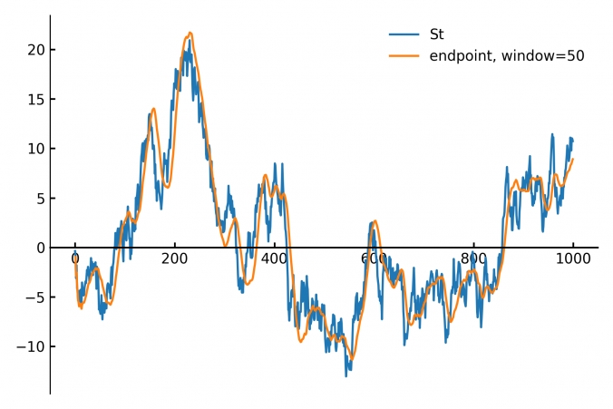
In finance and signal processing, detecting trends or smoothing noisy data streams efficiently is crucial. A popular tool for this task is a linear regression applied to a sliding (rolling) window of data points. This approach can serve as a low-pass filter or a trend detector, removing short-term fluctuations while preserving longer-term trends. However, naive methods for sliding-window regression can be computationally expensive, especially as the window grows larger, since their complexity typically scales with window size.
Fortunately, a clever algorithm—known in signal processing as the Savitzky-Golay filter—offers an efficient way to implement this sliding linear regression with constant-time complexity, independent of the window size. The key is to maintain a small set of running accumulators that update quickly at each new data point, resulting in O(1) complexity per update.

Below, we outline the mathematics behind this efficient streaming algorithm.
Ordinary Least Squares (OLS) Fit Equations
Given n pairs of data points  , we define the following summations:

The OLS solution for the line  is given by:

Sliding the Window Efficiently (O(1) Complexity)
To achieve constant-time complexity, we use the special case where the  -values are fixed integers
 ![x=[0, 1, \cdots, n-1]](https://www.sitmo.com/wp-content/ql-cache/quicklatex.com-c6edea12a88b2d25a69ca8bf0f8decba_l3.png "Rendered by QuickLaTeX.com") . In this scenario, two of the accumulators become constants:
. In this scenario, two of the accumulators become constants:
Only two accumulators need updating when sliding forward:
Updating  :
:
When the window slides forward one step, we receive a new value  and discard the oldest value
  . Thus, the update rule is:
![\[S_y^\prime \leftarrow S_y + y_n - y_0\]](https://www.sitmo.com/wp-content/ql-cache/quicklatex.com-b63fc0f77c5b1bd9da5d8856a8d6a771_l3.png "Rendered by QuickLaTeX.com")
For  , the update equation avoids recomputing the entire sum:
Initially we have:
![\[S_{xy} = 0 \cdot y_0 + 1 \cdot y_1 + 2 \cdot y_2 + \dots + (n-1) \cdot y_{n-1}\]](https://www.sitmo.com/wp-content/ql-cache/quicklatex.com-983937d41179c0282b8f68ae81d5ac7d_l3.png "Rendered by QuickLaTeX.com")
After sliding:
![\[S_{xy}^\prime \leftarrow 0 \cdot y_1 + 1 \cdot y_2 + \dots + (n-2) \cdot y_{n-1} + (n-1) \cdot y_n\]](https://www.sitmo.com/wp-content/ql-cache/quicklatex.com-ed69f41e6f021b11b0a062d0384aded5_l3.png "Rendered by QuickLaTeX.com")
Expressing  in terms of and
  :
:
![\[S_{xy}^\prime = S_{xy} - S_y^\prime + n y_n\]](https://www.sitmo.com/wp-content/ql-cache/quicklatex.com-f15e5dce55060c62acb20ffc6fca538e_l3.png "Rendered by QuickLaTeX.com")
This relationship requires only the previously computed accumulators and the new incoming value, providing constant-time complexity regardless of window length.
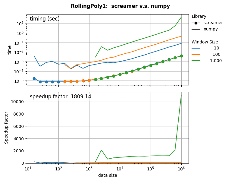
A C++ version of this algorithm in our screamer library executes 1mln linear regressions on streaming data, with a windows size 1000, in just 5 milliseconds. The speedup compared to numpy is a factor 1800, and against pandas 60.000.
Python code below!
from collections import deque
import numpy as np

class RollingLinearRegression:
    def __init__(self, window_size):
        """
        Implements an O(1) sliding window linear regression using a fixed-size rolling buffer.

        Parameters:
        - window_size: Number of points in the rolling window.
        """
        if window_size < 2:
            raise ValueError("Window size must be 2 or more.")

        self.window_size = window_size
        self.y_buffer = deque(maxlen=self.window_size)  # Ring buffer for y-values
        self.reset()  # Initialize all values

    def reset(self):
        """ Resets the accumulator values to their initial state. """
        self.y_buffer.clear()
        self.sum_y = 0.0
        self.sum_xy = 0.0
        self.n = 0  # Number of actual elements in the window
        self.sum_x = 0
        self.sum_xx = 0

    def add(self, yn):
        """
        Adds a new data point to the rolling window and updates regression statistics.

        Parameters:
        - yn: The new incoming y-value.
        """
        y0 = self.y_buffer[0] if len(self.y_buffer) == self.window_size else 0.0
        self.y_buffer.append(yn)

        self.sum_y += yn - y0

        if self.n < self.window_size:
            self.sum_x += self.n
            self.sum_xx += self.n * self.n
            self.sum_xy += self.n * yn
            self.n += 1
        else:
            self.sum_xy += self.window_size * yn - self.sum_y

    def get_slope(self):
        """ Returns the current slope (a) of the rolling regression line. """
        if self.n < 2:
            return None  # Not enough data points yet
        return (self.n * self.sum_xy - self.sum_x * self.sum_y) / (self.n * self.sum_xx - self.sum_x**2)

    def get_intercept(self):
        """ Returns the current intercept (b) of the rolling regression line. """
        if self.n < 2:
            return None  # Not enough data points yet
        slope = self.get_slope()
        return (self.sum_y - slope * self.sum_x) / self.n

    def get_endpoint(self):
        """
        Returns the estimated y-value at the last x-position (n-1),
        which can be used as a trend filter output.
        """
        if self.n < 2:
            return None  # Not enough data points yet
        slope = self.get_slope()
        intercept = self.get_intercept()
        return intercept + (self.n - 1) * slope